This book is Work in Progress. I appreciate your feedback to make the book better.

8.3 Latent Variables

Constructs, indicators, and measurement models

Some variables are comparatively straightforward to measure. Age can be taken from a register or asked directly. Income and number of children can be reported by respondents or recorded administratively. Their values may be missing, misreported, or defined differently across sources, but the variables are observable in principle.

Other concepts are less tangible and less naturally represented by one value. Happiness, risk attitude, personality, intelligence, and mathematical competence are examples. Yet none of them is automatically latent. Researchers sometimes measure such concepts with one direct question, sometimes with a score built from several items, and sometimes with a latent-variable model.

Every study must therefore make a measurement decision: how should a substantive concept become data? This process is called operationalization. A latent-variable model is one possible answer — an explicit model of how observed indicators relate to an unobserved quantity. It is not the only answer, and it is not automatically the best one.

The rest of this section builds that decision in four steps. First the vocabulary, once and in one place. Then three worked examples that form a ladder: a construct where one item is enough, a construct where several items are averaged, and a construct where a model is unavoidable. Only then the formal model and a map of the wider family.

8.3.1 How a Concept Becomes Data

Suppose you want to study happiness. You cannot put happiness into a regression. You can only put in a column of numbers, so something has to turn the concept into one. That step has a name — operationalization — and it is a decision, made by a researcher, that can be made well or badly.

The most direct route is to ask. A survey question produces a recorded response, and anything recorded in the data is an observed variable, sometimes called manifest. In measurement contexts the same response is also called an indicator, because it is being used as evidence about something rather than as an interesting quantity in its own right. Nothing mysterious has happened yet: a question was asked, an answer was written down.

Now notice what did not enter the data set. Happiness itself is nowhere in the file. Only an answer to a question about it is.

At this point a natural but wrong move is to call happiness unobserved and stop. Consider a genuinely unobserved value instead. A respondent skips the question about age, so that cell is empty. Age is unobserved for that person — and age has not become anything exotic. It is an ordinary variable with a gap, and the appropriate response is a missing-data method. The same goes for omitted variables and regression residuals: unobserved quantities, all of them, and none of them the thing this chapter is about.

The difference is not availability. It is whether a model represents the quantity. A variable is latent when it is not measured directly but is explicitly written into a statistical model, estimated through the indicators that are observed. Happiness is unobserved in the data either way. It becomes latent only when you build a model that contains it.

Which leaves one word for the thing itself, before any of these decisions: the construct — the substantive concept you are trying to study. A construct can be measured with one question, summarized by an average of several, or represented as a latent variable. All three are legitimate, and the choice is yours to justify.

Every latent variable is unobserved, but not every unobserved quantity is latent. Latentness is a modeling role, not a property of a concept.

This is why there is no fixed list of latent constructs. Happiness and personality are the textbook examples, and both are routinely measured with no latent variable anywhere in sight.

8.3.1.1 Reading a Path Diagram

One more convention before the examples, because these models are usually drawn rather than written. Three items measuring extraversion look like this:

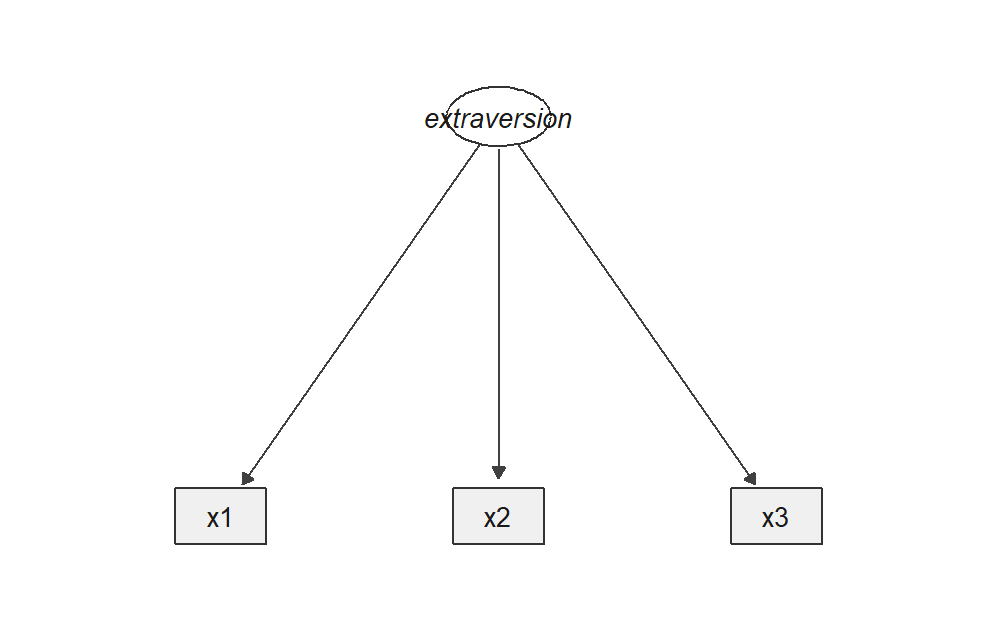
Figure 8.1: A latent variable with three indicators. The ellipse is not a column in the data; the rectangles are.

The grammar is small enough to state in full. A rectangle is an observed variable — a column that exists in your data. An ellipse is a latent variable, which is not. A single-headed arrow points from cause to effect; running from a factor to an indicator it is called a loading, written \(\lambda\), and it says how strongly that item responds to the construct. A double-headed arc between two ellipses is a covariance or correlation: the two are related, with no claim about which drives which. Each indicator also carries a small residual arrow, \(\varepsilon\), for the part of it the factor does not explain; these are omitted from most figures in this book to keep them readable.

One habit is worth forming immediately. The absence of an arrow is a claim too. Two factors drawn side by side with no arc between them are being asserted to be uncorrelated, and that assertion can be wrong.

8.3.2 One Item Can Be Enough: Happiness and Risk

Start with the case that measurement textbooks tend to skip.

The European Social Survey asks every respondent, in every round:

Taking all things together, how happy would you say you are? 0 = extremely unhappy … 10 = extremely happy⁹⁶

The German Socio-Economic Panel asks about life satisfaction in the same format:

How satisfied are you with your life, all things considered? 0 = completely dissatisfied … 10 = completely satisfied⁹⁷

And the Gallup World Poll — the data source behind the World Happiness Report — uses the Cantril ladder:

Please imagine a ladder with steps numbered from 0 at the bottom to 10 at the top. The top represents the best possible life for you, the bottom the worst possible life. On which step would you say you personally stand at this time?⁹⁸

Three single questions. Each produces one ordinary observed variable, and between them they support a large share of the empirical well-being literature and an annual international ranking of countries.

The same design appears for risk attitude. The SOEP asks whether respondents are generally willing to take risks or try to avoid them, from 0 to 10.⁹⁹ At the 2026 SOEP User Conference, Thomas Dohmen gave a keynote titled Twenty-Two Years of the General Risk Question,¹⁰⁰ which is the argument in one title: a single, carefully designed question can carry two decades of evidence when its target is clear, its wording is stable, and it is repeated across people, years, and countries.

Why one item is the right choice here. The construct is defined as a global self-assessment, and the question asks for exactly that. The item is not an imperfect proxy for something deeper — it is the outcome of interest. Beyond that, single items are cheap in respondent burden, can be repeated frequently in a broad panel, support comparison over time through stable wording, and can be validated against retests, external outcomes, and behavior.

When one item is not enough. A single response cannot separate the construct from item-specific measurement error, so its reliability cannot be estimated from itself. It cannot reveal whether the concept has several dimensions. And its interpretation depends on wording, response style, and the respondent's reading of the question.

That last limitation is not hypothetical, and the three questions above illustrate it. Happiness asks about affective state, life satisfaction asks for a cognitive judgment, and the Cantril ladder asks for a comparison against an imagined best possible life. They correlate substantially and they are not the same construct. Choosing one of them is a substantive decision, not a formatting detail.

A single item is a measurement model too — one with the loading fixed to one and the residual variance fixed to zero. Those are assumptions, not the absence of assumptions.

8.3.3 Several Items, One Score: The Big Five

Some constructs resist a single question because they are defined as broad domains.

Before the example, three instrument terms. An item is one question, statement, or task. A scale combines related items intended to measure one dimension, and a subscale is one scale inside a larger instrument. An inventory is a larger collection of items and scales describing several dimensions or facets. The usage is not perfectly rigid, but a practical distinction holds:

A scale usually produces one main score; an inventory produces a profile of several scores.

Personality shows why one item will not do. The Five-Factor Model distinguishes openness, conscientiousness, extraversion, agreeableness, and neuroticism. Each dimension is broader than any one statement: extraversion alone spans sociability, talkativeness, assertiveness, activity, and positive emotionality. Asking How extraverted are you? would collapse a facet structure that decades of psychological research established.

The NEO PI-3 takes that structure seriously. It contains 240 items and measures the five broad domains together with narrower facets underneath each.¹⁰¹ That number is worth pausing on: it is what a research programme looks like when it treats content coverage as the priority and can afford the testing time.

A general-purpose panel study faces the opposite constraint. The SOEP must also collect work, income, education, family, health, and housing information in the same interview. It therefore uses a short Big Five instrument with 15 items — three per dimension.¹⁰² This is not the NEO inventory mechanically truncated; it is a survey measure designed for a different purpose.

	NEO PI-3	SOEP BFI-S
Items	240	15
Resolution	five domains plus facets	five domains only
Cost	substantial testing time	a few minutes
Typical use	assessment, personality research	population panel, broad models

Fewer items mean less information and less precision per dimension. That is a trade-off to state, not a flaw to hide.

The usual analysis reverse-codes items pointing in the opposite direction and averages within a dimension. For three extraversion items:

\[ \text{Extraversion score}_p = \frac{x_{p1}+x_{p2}+x_{p3}^{\mathrm{reversed}}}{3}. \]

The result is an observed scale score: simple, transparent, and directly usable as a predictor or outcome. For many research questions it is entirely sufficient.

The same three responses could instead be treated as indicators of a latent extraversion factor. The difference is conceptual, not computational:

\[ \text{items}\longrightarrow\text{fixed average} \qquad\text{versus}\qquad \text{items}\longrightarrow\text{estimated latent factor}. \]

A fixed average assigns every item the same predetermined weight and treats the result as observed. A latent model estimates how strongly each item relates to the common factor and separates shared from item-specific variation.

More items make latent modeling possible; they do not make it mandatory. The inventory is the instrument. A scale score or a latent factor is an analytical representation built from it.

8.3.4 When a Model Is Necessary: Competence and Intelligence

The third rung is where the alternatives run out.

Asking How intelligent are you? measures self-assessed intelligence — a real and interesting variable, but not intelligence. Asking How good are you at mathematics? measures perceived competence, which reflects skill but also confidence, prior feedback, social comparison, and response style. No wording repair fixes this, because the construct is defined by performance and the question collects a judgment.

So switch to performance. One mathematics task records what a person actually did — but it still provides little evidence. A correct answer may reflect competence, a lucky guess, or prior familiarity with that specific problem. An incorrect answer may reflect lower competence, carelessness, a misreading, time pressure, or one unsuitable task.

This is why PISA, VERA, school and university examinations, and multi-stage assessment centres all take hours rather than minutes:

\[ \text{many tasks} \longrightarrow \text{response pattern} \longrightarrow \text{estimated competence}. \]

Four reasons make the length necessary:

1. Content coverage — tasks sample different parts of the intended domain.
2. Precision — isolated guesses, slips, and task-specific effects lose influence.
3. Range — tasks of varying difficulty inform about people at different competence levels.
4. Comparability — a measurement model places persons and tasks on one common scale.

In PISA 2022, the cognitive assessment lasted two hours per student, typically about 60 minutes of mathematics plus 60 minutes in another domain. The international item pool was far larger, so different students completed different but overlapping task sets.¹⁰³ That design buys broad coverage without asking any student to do everything — and it means raw counts of correct answers are not directly comparable across students. Item response theory exists to solve exactly that problem, and returns later in this chapter.

Intelligence testing follows the same logic, and it is where the whole method began. In 1904 Charles Spearman noticed that schoolchildren's marks in unrelated subjects — classics, French, mathematics, pitch discrimination — were all positively correlated. Nobody is good at everything by coincidence. Spearman proposed that one common cause, which he called general intelligence or g, accounted for the shared part, while each subject retained its own specific ability. To argue this, he had to invent factor analysis.

That pattern of uniformly positive correlations among cognitive tests is still called the positive manifold, and it remains one of the most replicated findings in psychology. What it does not settle is what \(g\) is. A single common factor is one explanation for a positive manifold; several correlated abilities are another; mutual reinforcement between abilities during development is a third. The statistical model is compatible with all three.

Even in this best case, then, the factor is not identical to the full theoretical concept. It is a model-based representation supported by one particular set of indicators — which is why the arrangement of the latent variables is itself a substantive claim, and the subject of the next section.

Single items, composite scores, and latent variables are alternative representations, not a hierarchy from inferior to superior.

The right choice depends on the construct, the research question, the precision required, the available survey or testing time, and the assumptions the researcher is willing to defend.

8.3.5 How Many Latent Variables?

Two questions arise once the notation is in place. How few indicators can a factor survive on, and how are several factors arranged relative to one another?

8.3.5.1 The Smallest Possible Factor Model

Start at the bottom. What does one factor with a single indicator look like?

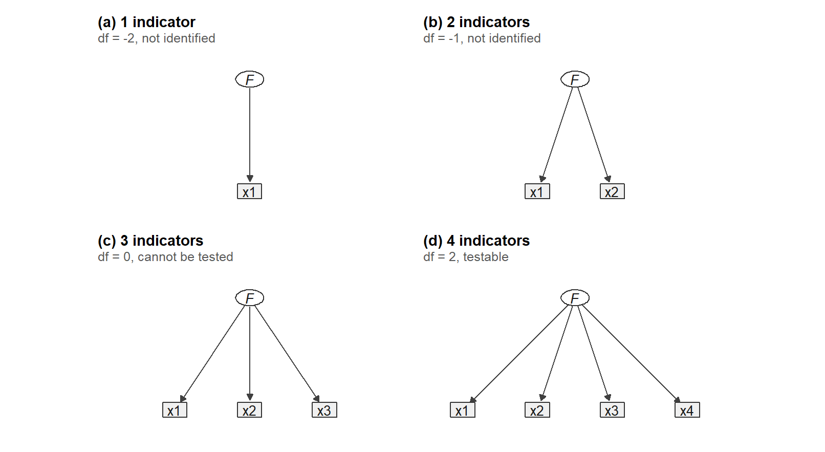
Figure 8.2: Growing a one-factor model one indicator at a time. Only the fourth is testable.

It looks perfectly reasonable, and it is useless. To see why, we need to know what the arrow actually stands for.

Write the model for one item:

\[ x_{i} = \nu_i + \lambda_i\,\eta + \varepsilon_i . \]

This is a regression — with one unusual feature: the predictor is not in your data. Everything else is familiar. \(\nu_i\) is an intercept. \(\lambda_i\), the loading, is a slope: how many points item \(i\) moves when the construct moves by one unit. And \(\varepsilon_i\) is a residual in exactly the ordinary sense — the part of the item the construct fails to account for, containing measurement error and whatever else is specific to that question.

Three quantities in that equation are unknown and must be estimated:

• the loading \(\lambda_i\) — the strength of the connection between construct and item;
• the factor variance \(\psi = \operatorname{Var}(\eta)\) — how much people differ on the construct. This one is peculiar, because the construct has no natural unit: nothing tells you whether extraversion is measured in points, kilograms, or anything else. So \(\psi\) is normally fixed to 1 by convention, or one loading is fixed to 1, purely to give the factor a scale;
• the residual variance \(\theta_i = \operatorname{Var}(\varepsilon_i)\) — how much of the item is not explained.

Now take variances on both sides of the equation. Because \(\eta\) and \(\varepsilon_i\) are assumed unrelated, the item's variance splits cleanly in two:

\[ \operatorname{Var}(x_i) \;=\; \lambda_i^{2}\,\psi \;+\; \theta_i . \]

That single equation is the whole of factor analysis in miniature: observed variance equals explained variance plus residual variance, exactly as in regression.

And it is also the problem. A model can only be estimated from the variances and covariances your data actually supply — with \(q\) observed variables there are \(q(q+1)/2\) of them. Subtract the free parameters and what is left is the degrees of freedom.

With one indicator the data supply exactly one number: \(\operatorname{Var}(x_1)\). The equation above has three unknowns on the right. One equation, three unknowns, and no sample size on earth will fix it. To make it estimable you must fix the loading to one and the residual variance to zero — at which point the "latent" variable is numerically identical to the item, just drawn as an ellipse. This is precisely the point made in Section 8.3.2: a single item is a measurement model, one whose assumptions are hidden by being invisible.

Two indicators add a covariance, and the covariance is where a common factor first leaves a trace: \(\operatorname{Cov}(x_1,x_2) = \lambda_1\lambda_2\psi\). Two items now supply three numbers — two variances and one covariance — against four unknowns once \(\psi\) is fixed (\(\lambda_1, \lambda_2, \theta_1, \theta_2\)). Still one short. A two-indicator factor becomes estimable only inside a larger model, or by forcing the two loadings to be equal — an assumption theory rarely supports.

Three indicators give six numbers — three variances and three covariances — against six unknowns (\(\lambda_1..\lambda_3, \theta_1..\theta_3\)). Everything is estimable and \(df = 0\): the model reproduces the observed covariances exactly, by construction. It cannot misfit, so its fit tells you nothing. A CFI of 1.000 here is arithmetic, not evidence.

Four indicators give ten numbers for eight unknowns, so \(df = 2\). Only now can the data contradict the model. This is why the rule of thumb says three indicators to estimate and four to test, and why the SOEP's three-item personality scales are perfectly usable as scores but cannot have their one-factor structure tested item by item.

Fixing a parameter is not a neutral technical step — it is the difference between a claim that can fail and one that cannot. A model with \(df = 0\) is a description; a model with \(df > 0\) is a hypothesis.

8.3.5.2 Five Arrangements

With enough indicators, the remaining question is how the latent variables relate to each other. Five arrangements cover most of what you will meet.

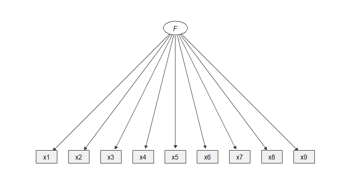
Figure 8.3: (a) One common factor: every indicator loads on a single latent variable.

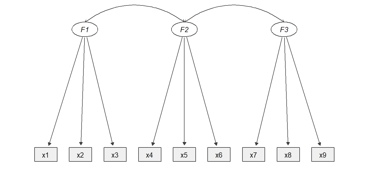
Figure 8.4: (b) Correlated factors: distinct factors, related to one another.

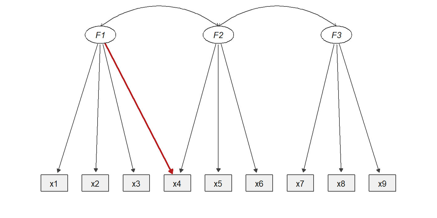
Figure 8.5: (c) A cross-loading: x4 is influenced by F2 as intended, and also by F1.

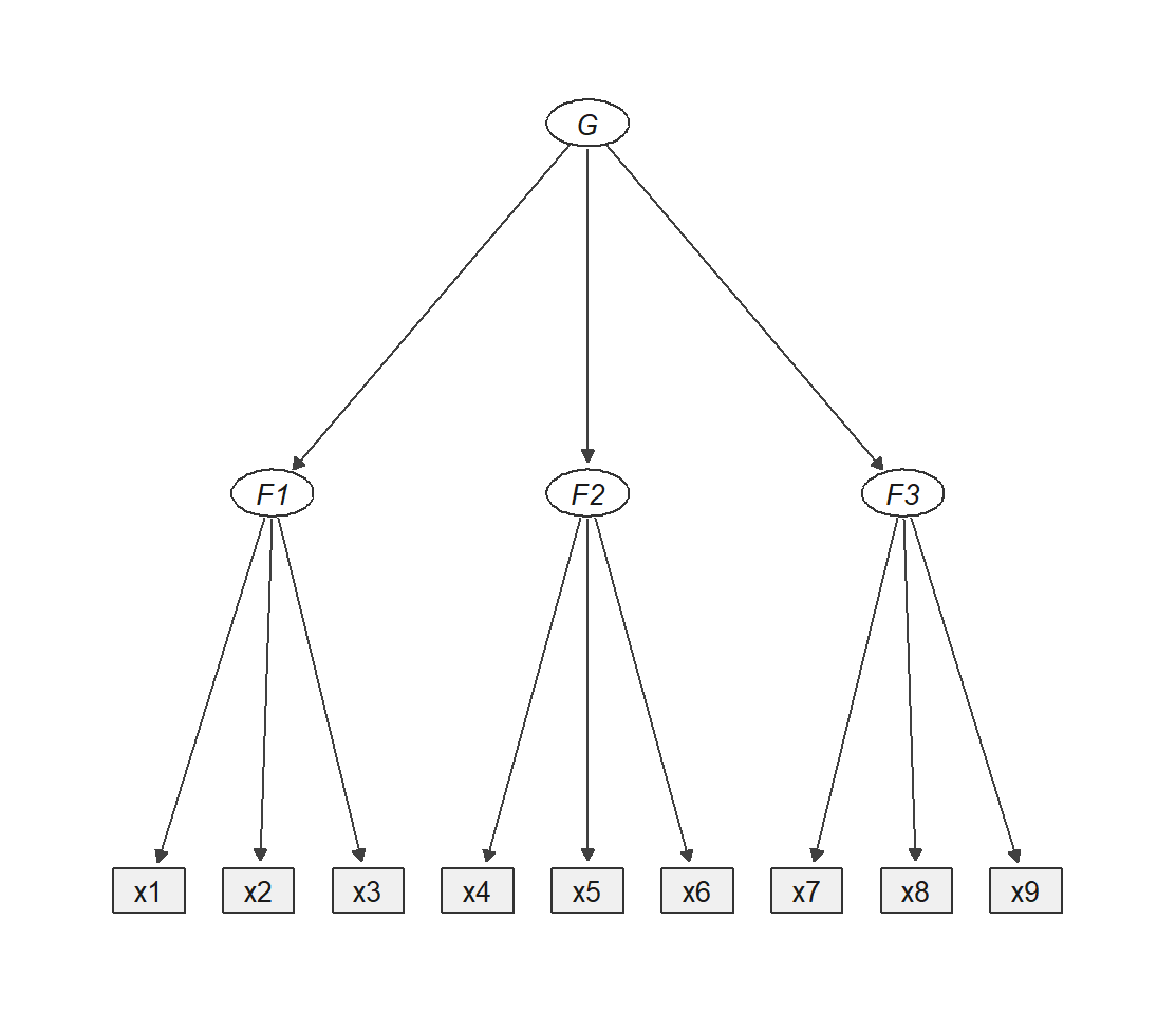
Figure 8.6: (d) Second-order factor: G reaches the indicators only through F1, F2 and F3.

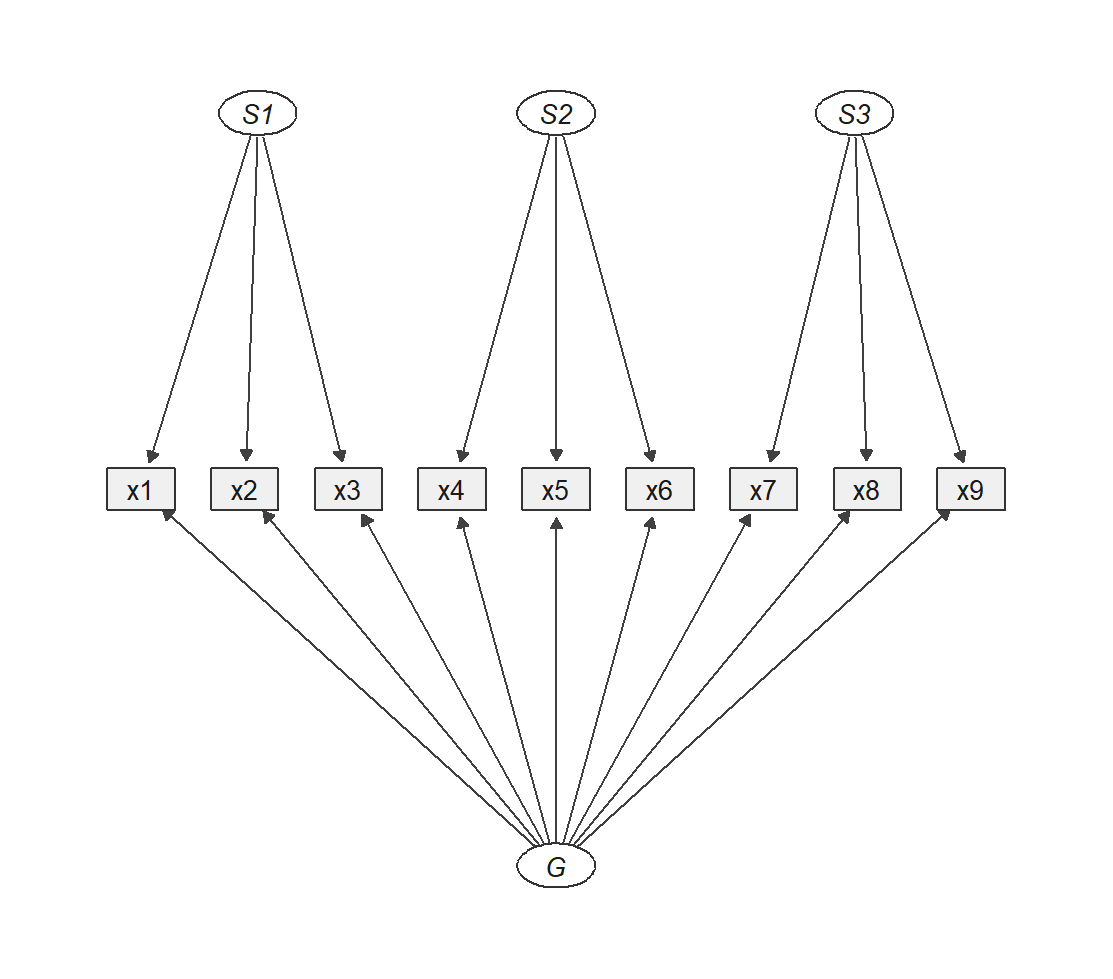
Figure 8.7: (e) Bifactor model: G loads on every indicator directly. No arcs, so G and each S are uncorrelated.

The letters mark genuinely different roles. F is a common factor for its own indicators, and it carries everything those items share. G is a general factor spanning every indicator in the model. S is a specific factor: what its group of items still shares after G has been accounted for.

So F1 and S1 are not the same object, even when they point at the same three items. In panel (b), F1 is the only common cause of x1–x3. In panel (e), G has already taken the variance common to all nine, and S1 is only what remains within x1–x3 on top of that. A specific factor is a residual common factor — which is why S loadings are usually smaller than the corresponding F loadings, and can even change sign.

In panel (a) the single factor is labelled F because that is its structural role. In intelligence research this same shape is the historical g from Section 8.3.4: the name is substantive, the shape is generic.

Panel (c) shows a cross-loading — a second arrow arriving at one indicator from a factor that is not its own. Here x4 is influenced by F2 as intended and by F1. Nothing about the picture is exotic; the claim is that one item measures two things at once. That happens when item content genuinely spans two domains, when wording is ambiguous, or when too few factors were retained. It is not automatically an error: the conventional model, which fixes every non-target loading to zero, is a strong restriction that item content does not always respect.

Panels (d) and (e) are the pair that gets confused. In the second-order model, G reaches the indicators only through the first-order factors — its job is to explain why F1, F2 and F3 correlate. In the bifactor model, G points at every indicator directly and is mediated by nothing, so each item carries two loadings. Note what is missing from panel (e): there are no arcs among G, S1, S2 and S3. In the standard bifactor specification those factors are constrained orthogonal, and that constraint is what makes "the general part of x1" and "the domain-specific part of x1" separable at all. Drop it and the model usually stops being identified.

A bifactor model also contains many more loadings than the alternatives, so it can fit well for reasons unrelated to being correct — exactly the situation the model-fit chapter of this book is about.

The number and arrangement of latent variables is a substantive hypothesis. Model fit can tell you that an arrangement reproduces the data poorly. It cannot tell you that a well-fitting arrangement is the right explanation.

Section 8.5 returns to these models with specification, identification, and estimation. Here they serve a narrower purpose: to show that "the latent variable" in a path diagram may be one bubble, several side by side, or several stacked in layers.

8.3.6 What a Latent Model Does

For continuous indicators, a basic one-factor measurement model is

\[ x_{pi} = \nu_i + \lambda_i\eta_p + \varepsilon_{pi}, \]

where \(x_{pi}\) is person \(p\)'s response to indicator \(i\); \(\nu_i\) is the indicator's intercept; \(\lambda_i\) its loading on the latent variable; \(\eta_p\) person \(p\)'s latent standing; and \(\varepsilon_{pi}\) indicator-specific residual variation.

The model explains associations among indicators through their shared relation to \(\eta\). It never observes \(\eta\). It proposes that a smaller unobserved structure can account for systematic patterns in observed data:

\[ \text{observed variation} = \text{shared factor variation} + \text{indicator-specific residual variation}. \]

Compared with a fixed average, the model can let indicators contribute unequally, retain residual variation instead of averaging it away, and quantify uncertainty. None of this is automatic. The interpretation depends on which indicators were selected, how the model was specified, and which assumptions connect indicators to the proposed construct.

A latent factor should therefore not be called the true construct, and residual variation should not be dismissed as meaningless noise.

8.3.6.1 Is the Latent Variable Ever Computed?

A natural question at this point is whether the estimation eventually produces a value of \(\eta_p\) for each person — a new column to be added to the data set. It does not.

What the model estimates are the loadings, intercepts, residual variances, and factor variances and covariances. The latent variable itself is integrated out: the entire model is fitted to the covariance matrix of the indicators. The practical demonstration is that a confirmatory factor model can be estimated from a covariance matrix and a sample size alone, with no individual responses at all, and the parameter estimates are identical to those obtained from the raw data. Nothing person-specific enters the estimation.

The circle in the path diagram is therefore exactly what it appears to be: a quantity in the model, not a column in the data.

Factor scores can be predicted afterwards as a separate post-hoc step — lavPredict() in lavaan offers several methods for this. Such scores are estimates with their own uncertainty, and different methods give different values for the same person, so they are not simply "the" latent values. They are not required for anything in this chapter, and structural equation modeling in particular relates latent variables to one another inside the model, without ever scoring a person.

There is one setting where person-level values genuinely are produced, and it is worth naming here because it looks like a contradiction. Large-scale assessments such as PISA do report competence on a scale, and item response theory does place each student on it. Even there, however, a single point estimate is avoided: PISA reports plausible values, several random draws from each student's posterior distribution, precisely because the student's competence remains uncertain after the test. Section 8.7 takes this up.

A latent variable becomes tangible through its loadings and through the covariance pattern it explains — not through a column of person values. Where person values are unavoidable, honest practice reports a distribution rather than a number.

8.3.7 A First Map of Latent-Variable Models

Two questions give a useful first orientation: is the latent variable continuous or categorical, and are the indicators continuous or categorical?

	Continuous indicators	Categorical indicators
Continuous latent variable	exploratory and confirmatory factor models	categorical factor models, Rasch models, item response theory
Categorical latent variable	latent profile and continuous mixture models	latent class models

The map is an orientation, not a taxonomy. Indicators may be ordinal, binary, counts, continuous, or mixed; models can combine continuous factors with latent classes, add repeated measurements or multiple levels, and use response distributions that fit no cell cleanly.

Structural equation modeling is deliberately absent, because it answers a different question: does the model only describe measurement, or does it also specify regressions and paths among variables?

The following sections follow one branch in depth:

\[ \text{explore a factor structure} \longrightarrow \text{specify and evaluate it} \longrightarrow \text{relate latent variables to other variables}. \]

• Exploratory factor analysis asks what common dimensions may be present.
• Confirmatory factor analysis states and evaluates an explicit measurement model.
• Structural equation modeling adds regressions and paths to measurement models.
• Item response theory focuses on categorical task responses, person competence, and item properties.

Two neighboring methods answer different questions. Principal component analysis builds weighted combinations of observed variables without positing latent causes or measurement error. Cluster analysis groups similar observations rather than measuring a continuous trait.

Latent-variable modeling is not one technique. It is a family of models distinguished by the observed evidence, the type of latent variable, and the relations imposed between them.

---

96. European Social Survey, core questionnaire, subjective well-being module (variable happy): https://www.europeansocialsurvey.org/methodology/ess-methodology/source-questionnaire.↩︎

97. SOEPcompanion, Life Satisfaction: https://companion.soep.de/Survey%20Design/Life%20Satisfaction.html.↩︎

98. Gallup World Poll item used in the World Happiness Report; see the report's statistical appendix on the Cantril ladder: https://worldhappiness.report/.↩︎

99. SOEPcompanion, Risk Aversion: https://companion.soep.de/Survey%20Design/Risk%20Aversion.html.↩︎

100. DIW Berlin, SOEP 2026 -- 16th International German Socio-Economic Panel User Conference, conference program and keynote announcement: https://www.diw.de/en/diw_01.c.982228.en/events/soep_2026_____16th_international_german_socio-economic_panel_user_conference.html.↩︎

101. PAR, NEO Personality Inventory-3: https://www.parinc.com/products/NEO-PI-3-NU.↩︎

102. SOEPcompanion, Personality -- Big Five: https://companion.soep.de/Survey%20Design/Personality%20%E2%80%93%20Big%20Five.html.↩︎

103. OECD, PISA 2022 Results, Volume II: https://www.oecd.org/en/publications/pisa-2022-results-volume-ii_a97db61c-en/full-report/component-7.html.↩︎