This book is Work in Progress. I appreciate your feedback to make the book better.

9.1 Experiments

Randomisation, natural experiments, and identification strategies

Section 5.3 left Ronald Fisher at Rothamsted with eight cups of tea and a promise: that the tea test was the smaller of the two things he built there. This is the larger one.

Before Fisher, agricultural trials were laid out in tidy systematic patterns — manure on the left strips, mineral nitrogen on the right — because tidiness looked like rigour. Fisher's argument was that the allocation should instead be decided by a physical act of chance, and that this act is not a concession to sloppiness but the thing that licenses everything the statistician does afterwards. His own chapter headings put it plainly: the interpretation of an experiment has a reasoned basis, and randomisation is the physical basis of the validity of the test.¹⁴⁵ Randomisation does two jobs at once. It severs the link between the treatment and every property of the plot — the drainage, the weeds, the slope, the things nobody measured and nobody thought of. And it manufactures the probability distribution against which the observed difference is judged.

That second point is worth pausing on, because it is the cleanest statement of what this whole chapter is about. In a randomised experiment, the p-value is not an assumption about nature. It is a fact about the coin.

Definition

Randomisation is the allocation of units to treatment and control by a chance device — a coin, a shuffled deck, a table of random numbers — rather than by the judgement of the researcher, the preference of the participant, or any rule connected to the units themselves.

Its power is not fairness. It is that chance is independent of everything: of the characteristics you measured, of the ones you did not, and of the ones nobody has yet thought to name. That independence is what lets a difference in outcomes be read as an effect. It is also what supplies the reference distribution against which the p-value is computed.

Note what randomisation is not. It is not a large sample, it is not a representative sample, and it is not haphazard allocation. Alternating patients by day of admission, or letting the field worker decide, produces something that looks arbitrary and is not random at all.

Most social scientists almost never get to use it. Economics has it worst, but sociology, political science, demography and any psychology that leaves the laboratory are all in the same position: the interesting causes are not ours to assign. The rest of this section is about what is done instead — and about the vocabulary invented for the problem, which is the vocabulary the following four sections take for granted.

9.1.1 The Problem Every Causal Question Has

Start with one person and one question. She completed a training programme and now earns €2,400 a month. Did the programme do that?

To answer it you would need one number that does not exist: what she would be earning today had she not enrolled. That world was never run. Every causal claim ever made is a comparison with a world that did not happen, and the missing half of the comparison is missing not by carelessness but by the structure of reality.

Paul Holland named this in 1986: the fundamental problem of causal inference.¹⁴⁶ Seen from this book's angle it is a missing-data problem of the most extreme kind. Section 4.1 dealt with values that are absent because somebody declined to answer; here the absent value never existed at all, and no amount of care in the fieldwork would have produced it. Half of every row is missing, always, by construction.

So we substitute. We find other people — who did not enrol — and let their earnings stand in for the world she did not live. That single move is the whole of causal inference, and everything that follows in this chapter is an argument about when the substitution is defensible.

Every method in this chapter answers one question, and it is worth memorising in this form: why should I believe that the untreated group shows me what would have happened to the treated group?

If you can state the answer in two sentences that a sceptical colleague would accept, you have a research design. If you cannot, you have a table of correlations with causal words attached.

Your Turn

Holland's fundamental problem, in your own words first.

For a person who enrolled, which of the two potential outcomes is observed? \(Y(1)\), the outcome under treatment\(Y(0)\), the outcome without itbothneither

Seen as a missing-data problem, what share of the potential-outcome table is missing, always? per cent.

Section 4.1 distinguished missing values that could in principle have been recorded from ones that could not. Which kind is a counterfactual? MCARMARneither - it was never a value that any fieldwork could have collected

And the sentence to memorise. Every method in this chapter answers one question. Which? which estimator is most efficient?why should I believe the untreated group shows what would have happened to the treated group?how large is the sample?

9.1.2 The Gold Standard, and Who Built It

There is exactly one construction in which the substitution needs no defence: decide who is treated by chance. Then the treated and untreated groups differ only by the accidents of the draw, so the untreated group is, in expectation, precisely the world the treated group did not live.

Definition

In a randomised controlled trial (RCT) the researcher allocates units to treatment and control by a chance device, measures the outcome in both arms, and reports the difference. A field experiment does this outside the laboratory, in the setting where the behaviour actually occurs; a laboratory experiment does it under controlled conditions; a survey experiment randomises something inside a questionnaire, such as the wording of a question or the description of a person.

It is called the gold standard because it is the only design that requires no argument about why the groups are comparable. That is a large claim, and it is narrower than it sounds: it holds for the people the trial was run on, in the place and period it was run. Whether the number means anything anywhere else is a separate question, and one no amount of randomising can answer.

The idea is younger than statistics and older than econometrics, and it did not begin in agriculture.

Psychology got there first. In 1885 Charles Sanders Peirce and Joseph Jastrow published a psychophysics memoir on whether people can perceive very small differences in pressure.¹⁴⁷ To keep the subject from anticipating anything, they took a pack of 25 cards — twelve red and thirteen black, reversed at the next sitting so that each colour was used 25 times across the 50 trials — shuffled it, and let the colour decide the order in which the two pressure changes were applied; a screen prevented the subject from seeing the operator's movements at all. Stephen Stigler judges it one of the earliest explicit endorsements of mathematical randomisation as a basis for inference — half a century before Fisher, and, in Stigler's own words, with the same what and why.¹⁴⁸ Read the fine print, though: Peirce and Jastrow randomised the order of conditions within one person, not the assignment of people to groups. Random group composition is a separate and later invention — the historian Trudy Dehue traces it to educational research in the 1920s — and the step between the two is bigger than it looks.¹⁴⁹

Fisher made it a principle. The requirement appears in Statistical Methods for Research Workers in 1925 and is argued at length in the 1926 field-experiments paper, where the instruction is to arrange the plots deliberately at random so that no distinction can creep in between plots treated alike and plots treated differently.¹⁵⁰ The Design of Experiments (1935) is where it becomes a book.

Medicine made it a rule. In 1931 Amberson, McMahon and Pinner split 24 tuberculosis patients into two matched groups of twelve and tossed a single coin to decide which group got the drug — one flip, two clusters, which is randomisation in spirit rather than in force.¹⁵¹ The trial usually called the first modern one is the Medical Research Council's streptomycin study of 1948, designed with Austin Bradford Hill: allocation was individual, drawn from random-number series prepared per sex and per hospital, and — the decisive innovation — sealed in envelopes so that no investigator could see what came next.¹⁵² Concealment, not arithmetic, is what made it credible.

Social science followed slowly. The first large-scale randomised social experiment was the New Jersey Graduated Work Incentive Experiment, which between 1968 and 1972 enrolled about 1,357 families and offered the treatment arms a guaranteed income, to find out whether it would stop them working.¹⁵³ Development economics arrived last and loudest: the Poverty Action Lab was founded at MIT in 2003, and the field experiment in the next subsection is one of thousands that followed.¹⁵⁴

The gold standard was coined by a sceptic

The phrase itself is remarkably recent. Historians of medicine trace its first application to randomised trials to a 1982 article in the New England Journal of Medicine by Alvan Feinstein and Ralph Horwitz — who used it to complain.¹⁵⁵ Their sentence was that epidemiological research matters precisely because it "offers a substitute for the unattainable scientific gold standard of a randomized experimental trial" — an elusive ideal, as the historians who dug the phrase out of the archive put it, invoked to dismiss observational evidence that is often all anyone has. The label had begun to do the work of an argument.

Forty years later the phrase is repeated in every methods course as though it settled something. It settles exactly one thing — that the comparison is fair — and leaves open everything else: whether the right question was asked, whether the right people were in the room, and whether the answer travels.

Your Turn

Four allocation schemes. Only one is randomisation.

patients are alternated by day of admissionthe field worker decides who looks most in needa random-number series is drawn in advance and sealed in envelopesthe first hundred volunteers are treated

The MRC streptomycin trial of 1948 is usually called the first modern randomised trial. Its decisive innovation was the statistical analysisconcealment - nobody could see what came nextthe sample sizethe placebo.

Amberson and co-authors tossed one coin to allocate two matched groups of twelve. How many independent randomisations is that?

True or false: randomisation guarantees that the treated and untreated groups are balanced on every measured covariate in the sample you actually drew. TRUEFALSE

9.1.3 The Catalogue of Designs

When the coin is not yours to flip, there are not very many alternatives. Almost everything in applied social science is one of the following, or a combination of two, and it is worth seeing the whole list before meeting any of them in detail.

Where the variation comes from	The claim you must defend	Design	Where in this book
A coin you flipped yourself	assignment is independent of the potential outcomes	randomised experiment	this section
Everything that drove selection was measured	conditional independence, given the covariates	matching, weighting, controls	Section 9.2
Repeated observation of the same unit	what is unobserved about a unit is fixed over time	fixed effects	Section 7.2
A date: something changed for one group only	the groups would have moved in parallel	difference-in-differences	Section 9.3
A threshold: a rule switches at a cut-off	everything else is continuous at the cut-off	regression discontinuity	Section 9.4
A lever that moves treatment and nothing else	relevance and exclusion	instrumental variables	Section 9.5

The order is not arbitrary. The designs are ranked by how much they ask you to believe about things you cannot see. Randomisation asks for nothing. Selection on observables asks for the most — that every driver of selection is sitting in your data set, an assumption that is untestable in principle and, as Section 9.1.7 will show on real data, sometimes spectacularly false. The designs in between buy their credibility by narrowing the comparison: to a period, to a neighbourhood of a threshold, to the people a lever happens to move.

A common misreading is that these are six ways of estimating the same number. They are not. A discontinuity design identifies an effect at the cut-off; an instrument identifies the effect for the people the instrument moves; difference-in-differences identifies it for the treated group in the treated period. Whose effect you end up with is a feature of the design, decided before the data are opened, and the honest write-up says so in the abstract.

9.1.4 Paying People to Learn Their HIV Status

In 2004, rural Malawi had a puzzle worth money. Door-to-door HIV testing was free and widely accepted, but the results were only available at a testing centre a few kilometres away, and most people never collected them. An untested guess about your own status is a bad basis for any decision. Rebecca Thornton ran an experiment: everyone tested was given a voucher, randomly drawn, worth between nothing and about three dollars, averaging around a dollar — roughly a day's casual wage — and redeemable only if they walked to the centre and asked for their result.¹⁵⁶

The data below are the teaching extract of her replication file.¹⁵⁷ One row is one person; got records whether they collected their result, any whether they received a voucher of any value, tinc the value in US dollars, distvct the distance to the centre in kilometres.

hiv <- read.csv(file.path("data", "Causal", "thornton_hiv.csv")) %>%
  rename(learned   = got,
         incentive = any,
         amount    = tinc,
         distance  = distvct,
         village   = villnum) %>%
  filter(!is.na(learned), !is.na(incentive))

nrow(hiv)
#> [1] 2834

The analysis is a difference of two means — the comparison of Section 5.2, unchanged and unadorned.

hiv %>%
  group_by(incentive) %>%
  summarise(n = n(), collected = mean(learned))
#> # A tibble: 2 × 3
#>   incentive     n collected
#>       <dbl> <int>     <dbl>
#> 1         0   623     0.339
#> 2         1  2211     0.789

Without a voucher, 34% came back for their result. With one, 79%. The gap is 45 percentage points in this extract, and it is the largest single behavioural response in this book.¹⁵⁸

t.test(learned ~ incentive, data = hiv)
#> 
#>  Welch Two Sample t-test
#> 
#> data:  learned by incentive
#> t = -21.593, df = 898.16, p-value < 0.00000000000000022
#> alternative hypothesis: true difference in means between group 0 and group 1 is not equal to 0
#> 95 percent confidence interval:
#>  -0.4915022 -0.4096015
#> sample estimates:
#> mean in group 0 mean in group 1 
#>       0.3386838       0.7892356

R subtracts the groups in label order, so it prints the difference as \(-0.451\) and the statistic as \(t = -21.6\); the sign is bookkeeping, the magnitude is the finding.

The crudest tool in the book

Look at what produced that number: t.test(), from Section 5.2, four chapters before any econometrics. No control variables, no specification search, no robustness appendix. The estimator is the crudest tool in this book, and it is sufficient, because all of the sophistication went into the design rather than into the analysis.

There is a general rule hiding in that, and it is worth carrying into every paper you read: the cleaner the source of variation, the simpler the analysis can be. A well-run experiment needs a difference in means. A sharp discontinuity needs a local comparison around a cut-off. A murky observational comparison needs matching, weighting, controls, fixed effects, clustering and a battery of specifications — and needs them precisely because the design cannot carry the claim on its own.

The inverse is a useful reading habit rather than a law. Methodological machinery is sometimes a sign of care and sometimes a sign that no single comparison was convincing enough to stand alone. When a paper's appendix is three times the length of its identification argument, it is worth asking which of the two is doing the persuading.

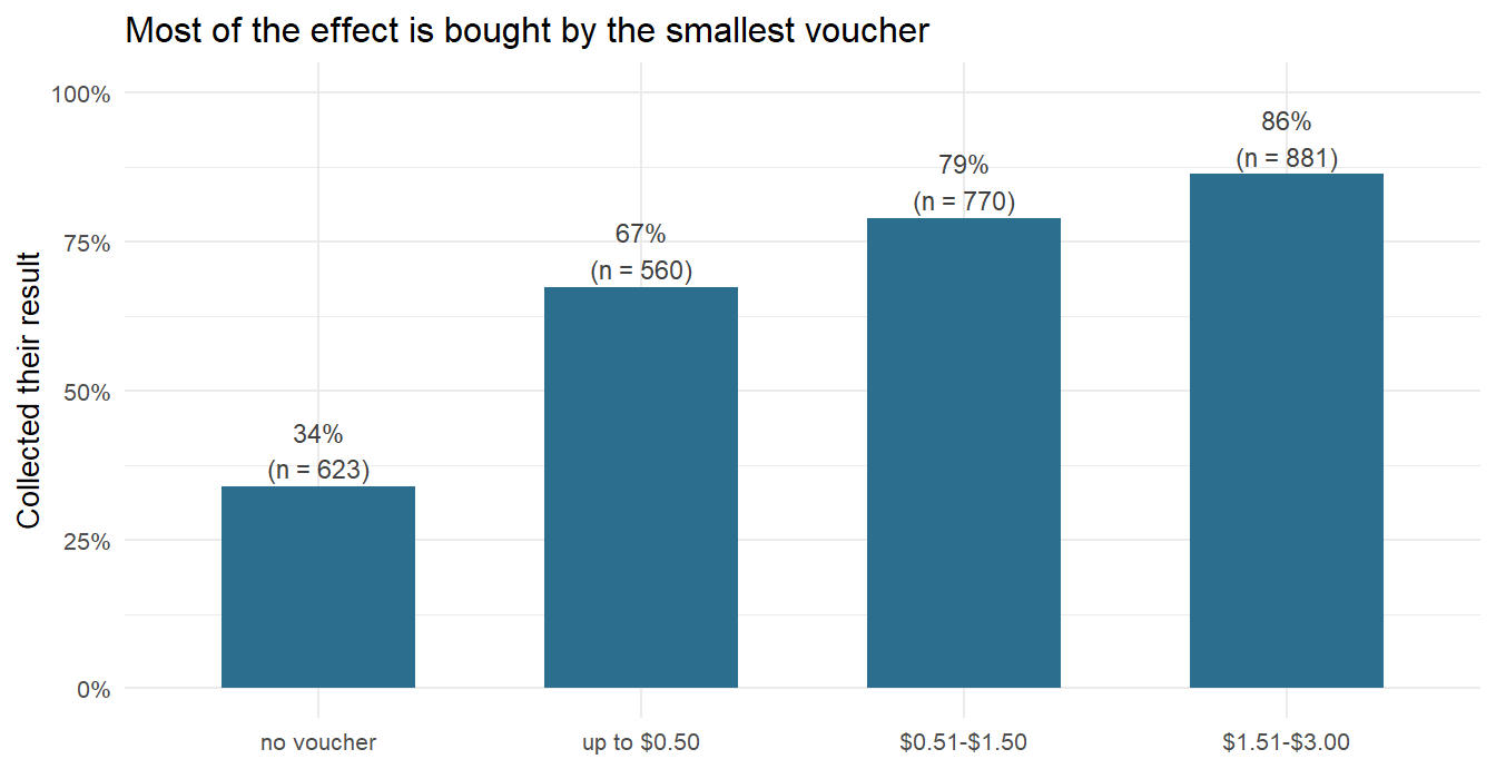
Figure 9.1: Share collecting their HIV result, by the value of the randomly assigned voucher. The jump from nothing to a token amount is far larger than any further increase — most of the effect is bought by the first few cents.

The dose-response pattern is the part economists find interesting, and it is only visible because the amount was randomised too. A voucher worth at most fifty cents already lifts collection from 34% to 67%; raising it to two dollars or more adds a further nineteen points. Thornton makes the same point in the paper: even the smallest amount, about a tenth of a day's wage, produced large gains. This does not look like people being paid for their time. It looks like a small nudge past a threshold — which is a hypothesis about mechanism, generated by the design rather than assumed by it.

Now the sanity check that every experiment owes its reader. If assignment was truly random, the groups should look alike on everything measured before the voucher was handed out.

hiv %>%
  mutate(hiv2004 = ifelse(hiv2004 < 0, NA, hiv2004)) %>%
  group_by(incentive) %>%
  summarise(n         = n(),
            age       = mean(age, na.rm = TRUE),
            distance  = mean(distance),
            hiv_positive = mean(hiv2004, na.rm = TRUE))
#> # A tibble: 2 × 5
#>   incentive     n   age distance hiv_positive
#>       <dbl> <int> <dbl>    <dbl>        <dbl>
#> 1         0   623  32.1     1.96       0.0629
#> 2         1  2211  33.7     2.03       0.0627

Distance and HIV status match almost exactly. Age does not: the voucher group is 1.6 years older, and a t-test puts that at \(p = 0.007\). This is not a scandal, and pretending otherwise would teach the wrong lesson. Randomisation balances groups in expectation, not in every realised sample; check ten pre-treatment variables and one will typically fail at the 5% level because that is what 5% means. The right response is not to abandon the experiment but to see whether the estimate cares.

lm(learned ~ incentive + age + distance, data = hiv) %>%
  summary() %>% coef() %>% round(4)
#>             Estimate Std. Error t value Pr(>|t|)
#> (Intercept)   0.3404     0.0276 12.3132   0.0000
#> incentive     0.4488     0.0192 23.4283   0.0000
#> age           0.0018     0.0006  3.0099   0.0026
#> distance     -0.0291     0.0062 -4.6516   0.0000

The coefficient moves from 0.451 to 0.449. In an experiment, control variables buy precision, not identification — and here they barely buy even that. Hold that number next to what control variables do in Section 9.1.7, where the design is not there to carry them.

One thing the balance table quietly understates. distance is not merely a background variable that happened to come out even: Thornton randomised the location of the results centres as well as the voucher, so distance is a second randomised arm. The design is richer than a single coin flip, and that is why the two columns agree on it to two decimal places.

The file also stores a small number of unusable HIV results as -1, which is exactly the pattern Section 4.1 warned about: a negative number that is not a quantity but a code, and that a mean will happily swallow. The ifelse() above is the two-second fix.

A second caveat on precision: vouchers were drawn within 119 villages, and people in the same village talk to one another. Allowing for that widens the standard error from about 0.019 to 0.023 and leaves the estimate untouched. Clustered standard errors return in Section 7.2.

Your Turn

Collection rates were 33.9% without a voucher and 78.9% with one.

The effect in percentage points is .

Suppose the vouchers had not been randomised — suppose instead that field workers handed them to whoever seemed least likely to come back. Would the naive difference then be too large or too small? too largetoo smallunchanged, because the outcome is binary

And the design question. Thornton randomised the voucher amount as well as its existence. What does that buy her that a simple treated-versus-untreated design would not? a larger samplea dose-response curve, which speaks to the mechanismprotection against selection bias, which randomising the existence alone does not give

9.1.5 What We Want and Cannot Have

Having seen one work, it is worth writing the logic down properly. The notation below is the common language of the whole field; it takes ten minutes to learn and it makes every later section shorter.

Definition

For unit \(i\) and a binary treatment \(D_i \in \{0, 1\}\), the two potential outcomes are \(Y_i(1)\), the outcome under treatment, and \(Y_i(0)\), the outcome without it. The causal effect for that unit is

\[\delta_i = Y_i(1) - Y_i(0)\]

What the data contain is only \(Y_i = D_i \cdot Y_i(1) + (1 - D_i) \cdot Y_i(0)\) — one of the two, never both. That is the fundamental problem of the previous subsection, written in four symbols.

Because individual effects are unknowable, causal work reports averages, and the naive comparison between the treated and the untreated splits cleanly into two pieces:

\[\underbrace{E[Y \mid D = 1] - E[Y \mid D = 0]}_{\text{what we compute}} \; = \; \underbrace{E[Y(1) - Y(0) \mid D = 1]}_{\text{the effect on the treated}} \; + \; \underbrace{E[Y(0) \mid D = 1] - E[Y(0) \mid D = 0]}_{\text{selection bias}}\]

The second term asks one question: would the two groups have differed anyway, with no treatment at all? Randomisation forces it to zero by construction. Every other design in this chapter is an argument for why it is zero, or small, or bounded, inside some deliberately narrowed comparison.

Truly Dedicated: whose average is it?

"The average effect" is three different quantities that routinely get confused, and the difference between them is not pedantry — policy conclusions turn on it.

The average treatment effect, \(\text{ATE} = E[Y(1) - Y(0)]\), is the effect if everybody were treated. It is what a minister usually has in mind when asking whether a programme works.

The average treatment effect on the treated, \(\text{ATT} = E[Y(1) - Y(0) \mid D = 1]\), is the effect for the people who actually took it. If people select into treatment because they expect to gain, the ATT is larger than the ATE, sometimes much larger — and it is the honest answer to "did this programme help its participants", not to "should we scale it up".

The local average treatment effect, LATE, is the effect for whoever a particular instrument or threshold happens to move. It returns in Section 9.5 and in the discussion of the credibility revolution at the end of this section.

Which of the three a study delivers is decided by its design, before any estimation. Randomising the whole eligible population gives the ATE. A voluntary programme evaluated against a comparison group gives the ATT. A discontinuity gives an effect at the cut-off and nowhere else.

Your Turn

Three quantities, three questions, and policy conclusions turn on the difference.

A minister asks "would this work if we rolled it out to everybody?" She wants the ATEATTLATE.

An evaluator asks "did this programme help the people who took it?" That is the ATEATTLATE.

If people select into treatment because they expect to gain, then the ATT is smaller thanlarger thanequal to the ATE.

Now the decomposition. The naive difference equals the effect on the treated plus selection bias. Randomisation forces the second term to by construction.

And the harder one. If a programme deliberately recruits the people doing worst, the naive comparison overstates the effectunderstates it, and can reverse its signis unaffected.

9.1.6 Why Economists Rarely Get to Randomise

The obvious obstacles come first. Nobody can randomise a recession, an exchange-rate regime, a minimum wage, a currency union, or a person's parents. Where an experiment is conceivable it is often forbidden, unaffordable, or too slow: the interesting outcomes in labour economics arrive twenty years after the intervention.

But there is a deeper reason, and it is close to the identity of the discipline. In most sciences, selection into treatment is a nuisance that contaminates the data. In economics it is the subject. People enrol in training because they expect it to pay off. Firms adopt a technology because it suits their workforce. Countries deregulate because of the circumstances that made deregulation attractive. The assignment mechanism is optimising behaviour, which is the thing the discipline exists to study — and this is why selection bias in economics is rarely small and rarely random in sign. The people who take the treatment are systematically the ones for whom it is worth taking.

Definition

Selection into treatment is the process by which units come to be treated at all. It is a fact about the world, and in an experiment it is a coin.

Self-selection is the particular case in which the units decide for themselves, on the basis of something they know about their own likely gain — a talent, a plan, a diagnosis, a family situation. It is the normal case outside the laboratory.

Selection bias is what these do to your estimate: the difference the two groups would have shown even with no treatment at all. It is the second term of the decomposition above, and it has a sign you can usually reason about in advance. If the people who enrol are the ones who expected to do well anyway, the naive comparison overstates the effect. If a programme deliberately recruits the people doing worst, it understates it — and can reverse it, as the next subsection shows on real data.

The three words are worth keeping apart. The first is a mechanism, the second is one form of it, and the third is the damage.

This is why "we controlled for the observable differences" is a weaker sentence than it sounds. If people choose treatment on the basis of an expected gain that they can see and you cannot, then the variable driving selection is by definition absent from your data set. No amount of controlling closes a gap you cannot measure.

So the answer to selection is not a better estimator. It is a better source of variation: some part of the treatment that moved for reasons having nothing to do with the people it moved. Finding one is what the next four sections are about, and what the rest of this section names.

9.1.7 LaLonde's Challenge

In 1986 Robert LaLonde had a data set nobody else could use the way he used it.¹⁵⁹ The National Supported Work Demonstration was a mid-1970s American programme offering nine to eighteen months of subsidised work experience to people with severe employment barriers: former offenders, former drug users, long-term welfare recipients, school dropouts. Crucially, it had more applicants than places, and it allocated them by lottery. It was a genuine randomised experiment on a question at the centre of labour economics.

LaLonde's move was not to analyse the experiment. It was to use the experiment as an answer key. Take the experimental estimate as the truth. Then throw away the randomised control group, replace it with a comparison group drawn from a national survey — the kind of comparison group econometricians actually had — and see whether the era's best methods could recover the known answer.

nsw <- read.csv(file.path("data", "Causal", "nsw_experimental.csv"))
cps <- read.csv(file.path("data", "Causal", "cps_controls.csv"))

c(treated = sum(nsw$treat == 1), randomised_controls = sum(nsw$treat == 0),
  cps_controls = nrow(cps))
#>             treated randomised_controls        cps_controls 
#>                 185                 260               15992

re78 is earnings in 1978, after the programme; re74 and re75 are earnings before it. The experimental estimate is the difference in 1978 earnings between the 185 people admitted and the 260 turned away by the lottery. Then the same 185 treated men are compared with 15,992 survey respondents instead.

Show the code that builds the table below.

obs <- bind_rows(nsw %>% filter(treat == 1), cps)

models <- list(
  "Experiment"        = lm(re78 ~ treat, data = nsw),
  "Survey controls"   = lm(re78 ~ treat, data = obs),
  "Survey + controls" = lm(re78 ~ treat + age + educ + black + hisp +
                             marr + nodegree + re74 + re75, data = obs)
)

modelsummary(models,
             coef_map = c("treat" = "Training programme"),
             gof_map  = c("nobs", "r.squared"),
             title = "The same 185 trained men, three comparison groups. Only the first column comes from a lottery.")

The same 185 trained men, three comparison groups. Only the first column comes from a lottery.

	Experiment	Survey controls	Survey + controls
Training programme	1794.342	-8497.516	699.132
	(632.853)	(712.021)	(547.636)
Num.Obs.	445	16177	16177
R2	0.018	0.009	0.476

The experiment says the programme raised annual earnings by about $1,794. Swap the randomised controls for the survey sample and the same programme appears to have cost its participants $8,498 a year. The sign is wrong, the magnitude is wrong, and the difference between the two numbers — over $10,000 — is pure selection bias, with exactly the sign the previous subsection predicted: the programme deliberately recruited the least employable people in America, and the survey sample is America.

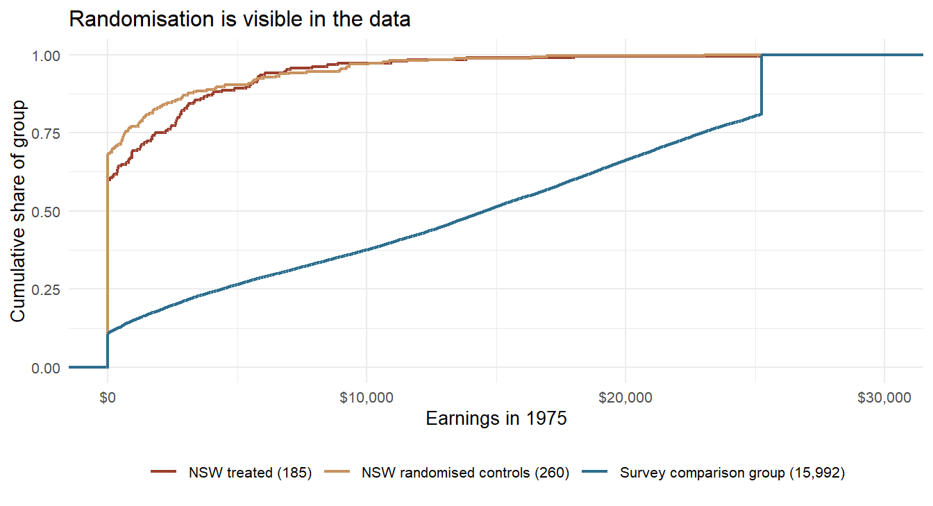
Figure 9.2: Earnings in 1975, before the programme, as cumulative shares. The two randomised groups lie almost on top of one another; the survey comparison group is a different population. Read off where each curve leaves the vertical axis: that is the share with no earnings at all. The blue curve's jump to one just below $26,000 is not behaviour, it is topcoding.

The figure is the point of the whole section. A randomised control group is not merely similar to the treated group; it is drawn from the same population by construction, and the two curves are indistinguishable before the treatment ever happens. The survey group is a different country.

Table 9.1: Pre-treatment characteristics. The first two columns were made comparable by a lottery; the third was not, and no column of numbers will make it so.

Variable	NSW treated	NSW control	Survey control
Age	25.82	25.05	33.23
Years of schooling	10.35	10.09	12.03
Black	0.84	0.83	0.07
Hispanic	0.06	0.11	0.07
Married	0.19	0.15	0.71
No high-school degree	0.71	0.83	0.30
Earnings 1974 (USD)	2095.57	2107.03	14016.80
Earnings 1975 (USD)	1532.06	1266.91	13650.80

The wrong estimate is not the imprecise one. It has 16,177 observations, a standard error of $712 and a t-statistic of nearly \(-12\). It is wrong by more than $10,000 and it is wrong with great confidence. Precision is not credibility. A large sample buys the first and none of the second — and the modern era of administrative data, with millions of rows, has made this failure mode cheaper than ever to produce.

Your Turn

The experiment says \(+\$1{,}794\). The survey comparison says \(-\$8{,}498\).

The gap between them is dollars, and every cent of it is selection bias.

Its sign was predictable in advance. Why? because the programme was expensivebecause the programme deliberately recruited the least employable people in America, and the survey sample is Americabecause 1978 earnings are noisy

Add the eight controls and the estimate becomes \(+\$699\): right sign, plausible magnitude, respectable standard error. Why is that the worst of the three outcomes? it is not - it is the best of the threebecause a referee would not blink, and nothing on the printout says it is less than half the right answerbecause the standard error is too large

True or false: an estimate built on 16,177 observations deserves more trust than one built on 445. TRUEFALSE

Now look at the third column of the table. Add the eight control variables — age, schooling, ethnicity, marital status, degree, and two years of prior earnings — and the estimate becomes +$699. The sign is right. The magnitude is plausible. The standard error is respectable. A referee would not blink. And it is less than half the experimental answer, with nothing on the printout to say so.

That was LaLonde's finding, and it landed hard: the econometric fixes of the day, applied honestly by a competent analyst, did not reliably recover an answer that was known. The literature has argued about it ever since. Rajeev Dehejia and Sadek Wahba showed in 1999 that propensity-score matching on a well-chosen subsample gets close to the experimental number, which is a large part of why matching became popular.¹⁶⁰ Jeffrey Smith and Petra Todd then showed how much that success depends on which subsample, which covariates and which specification.¹⁶¹ The debate is the reason Section 9.2 exists, and the reason it is the first of the four method sections rather than the most trusted.

9.1.8 Identification Is Not Estimation

The LaLonde comparison separates two ideas that beginners tend to fuse.

Definition

A parameter is identified if it could be recovered exactly from the data-generating process given an infinite sample, under the assumptions being made. Estimation is what remains after that: extracting the number from a finite sample, with sampling error attached.

An identification strategy is the argument for why a particular comparison in the data corresponds to the causal quantity of interest. It is a claim about how the world assigned the treatment — not a property of the model, the software, or the sample size.

No amount of data solves an identification problem. LaLonde's survey comparison had 16,177 observations and was wrong; the experiment had 445 and was right. More rows would have shrunk the standard error around the wrong number.

Truly Dedicated: two things economists call identification

Behind that definition sits a phrase worth owning: the data-generating process, the mechanism in the world that actually produced the numbers in front of you. Every method in this book is an attempt to say something about that mechanism while only ever seeing its output. Identification is the question of which parts of the mechanism the output can pin down at all, before any question of sample size arises.

Put that way, the word has a much older home in economics than treatment effects have. A market hands you a cloud of price-and-quantity pairs. Every point in it is the intersection of a supply curve and a demand curve, and both curves move. Fit a line through the cloud and you get neither of them — at best you trace out demand in the years when supply happened to do the moving. Elmer Working laid this out in 1927 in a paper whose title is still the best summary of the problem: What do statistical "demand curves" show?¹⁶² Trygve Haavelmo turned it into probability theory in 1943 and 1944, and Tjalling Koopmans gave the problem its name and its order and rank conditions in 1949.¹⁶³ From that tradition come the words under-identified, exactly identified and over-identified, and the reflex of counting equations against unknowns. It is still the meaning you meet first in a structural econometrics course, and it is still alive — agricultural economists identify supply and demand this way today, occasionally by exotic routes such as exploiting changes in the variance of the shocks rather than in their level.¹⁶⁴

The design-based meaning of this chapter is the same question asked of a different mechanism. Not which curve produced this point, but which comparison recovers this effect. Both ask what the observable distribution can and cannot pin down. Both are settled by assumptions rather than by data.

And both are best learned the way you may already have met them in R: write the data-generating process yourself, hide the formula, and see whether the method finds its way back to the numbers you chose. That is exactly what Section 4.2 does when it builds a data set by hand — and it is the only situation you will ever be in where the right answer is known.

This has a practical consequence that is worth stating bluntly. An identification strategy is stated in words, before it is stated in code, and it is checked by argument rather than by diagnostics. \(R^2\), t-statistics, information criteria and robustness tables all take the comparison for granted; none of them can tell you that the comparison was never causal to begin with. When you read an empirical paper, the identification strategy is what the introduction spends its third and fourth paragraphs on, and it is the only part that cannot be fixed in revision.

Your Turn

Sort each of these into identification or estimation.

"Given an infinite sample from this data-generating process, could the parameter be recovered exactly?" — that is identificationestimation.

"How much sampling error does my 4,000-row sample leave around the number?" — that is identificationestimation.

"Should I cluster the standard errors?" — that is identificationestimation.

"Is the untreated group a fair stand-in for the treated group's counterfactual?" — that is identificationestimation.

Which of the four can be fixed by collecting more data? all of themonly the estimation onesnone of them

And the older meaning, from the box above. A cloud of price-and-quantity pairs traces out a demand curve only when demand is doing the movingsupply is doing the movingboth are moving.

9.1.9 When the Design Runs Out

Four situations turn up constantly and are not on the catalogue's list. Naming them is part of the vocabulary.

The policy that hit everybody. A national reform, a currency changeover, a pandemic — there is no untreated group, because the treatment was the country. The usual answers are to build a comparison group rather than find one, which is what the synthetic control method does by weighting other regions into an artificial twin of the treated one,¹⁶⁵ or to compare against the treated unit's own past, which turns the problem into a time-series question. Both work. Both buy identification with an assumption stronger than anything in the catalogue, and the honest paper says which.

The lever that barely moves. An instrument that shifts the treatment only weakly is worse than no instrument at all: the estimate drifts back towards the biased comparison it was meant to fix, and the standard errors understate how little is known.¹⁶⁶ The familiar guard is the first-stage F-statistic and the rule of thumb that it should clear 10 — a benchmark from Staiger and Stock, formalised by Stock and Yogo, and by now widely thought too generous.

The treatment that spreads. Every design in the catalogue assumes that one unit's treatment does not change another unit's outcome. Vaccination breaks that. So does a training programme large enough to move local wages, and so does anything involving classmates, colleagues or neighbours. The special case where the group's average causes the individual and the individual is part of the average has a name of its own — Charles Manski's reflection problem — and it is genuinely unidentified, not merely difficult: you cannot tell the mirror from the person.¹⁶⁷

The question that was never causal. Some of the most useful numbers in the social sciences are accounting, not causation. How much of the gender wage gap corresponds to measured differences in occupation, hours and experience is an Oaxaca-Blinder decomposition — the subject of Section 6.3 — and it is an entirely respectable exercise as long as nobody calls the unexplained remainder "discrimination". A decomposition apportions a difference. It does not say what would happen if you changed something.

Two words worth separating for good. Internal validity asks whether the estimate is right for the people and the setting it was measured in. External validity asks whether it tells you anything about anywhere else. Designs buy internal validity by narrowing the comparison — to a threshold, a period, the people a lever moves — and every narrowing costs external validity. The trade is unavoidable; pretending it is not is the most common overreach in applied work, and it is the reason the gold standard of Section 9.1.2 is a narrower claim than the phrase suggests.

Your Turn

Four situations, four names. Match them.

A national currency changeover, with no untreated group anywhere: the reflection problemno comparison group - the usual escape is a synthetic controla weak instrumentan accounting exercise

A vaccination programme large enough that the untreated benefit too: no comparison groupthe reflection problema SUTVA violation - the treatment spreadsa weak instrument

A classroom in which the group average causes the individual and the individual is part of the average: a SUTVA violationthe reflection problem, which is genuinely unidentifiedselection bias

The share of the gender wage gap that corresponds to measured differences in occupation and hours: a causal effectan accounting exercise - a decomposition apportions a difference, it does not say what would changea weak instrument

And the pair that gets confused most. A study of one oversubscribed school's lottery has high internalexternal validity and low internalexternal validity.

9.1.10 Natural Experiments

Between the coin flip and the survey comparison sits the design that gave economics its modern shape.

Definition

A natural experiment is variation in treatment produced by nature, an institution or an administrative accident, which the researcher argues is as good as randomly assigned with respect to the outcome. The researcher does not assign anything. The researcher finds an assignment that somebody else, or something else, already made — and then argues that it was made for reasons unrelated to the outcome.

A quasi-experiment is the same idea with the "as good as random" claim resting on a design feature rather than on chance: a threshold, a timing, an eligibility rule.

A short catalogue from economics, each of which is now a section in some textbook:

• The draft lottery. Birth dates were drawn from a drum to determine Vietnam draft eligibility. Joshua Angrist used the drawn numbers to isolate the effect of veteran status on later earnings — the lottery moved military service, and nothing else about a man depended on his birth date.¹⁶⁸
• Quarter of birth. Compulsory schooling laws tie the leaving date to a birthday, so children born in different quarters were forced to complete different amounts of schooling. Angrist and Alan Krueger used this to estimate the returns to education.¹⁶⁹
• The Mariel boatlift. In 1980, 125,000 Cubans arrived in Miami within five months. David Card treated it as a labour-supply shock that no Miami employer or worker had chosen, and asked what it did to local wages.¹⁷⁰
• A state border. New Jersey raised its minimum wage in 1992; Pennsylvania did not. Card and Krueger surveyed fast-food restaurants on both sides.¹⁷¹
• An actual government lottery. Oregon could not afford Medicaid places for everyone eligible in 2008, so it drew names. The result is a randomised experiment on health insurance that no researcher had to design.¹⁷²
• A wall. German reunification remains one of the most-used natural experiments in European economics, and much of that work runs on the household panel this book keeps returning to in Section 2.2.

The first natural experiment

London, 1854. Two companies piped water into the same streets, sometimes into neighbouring houses. Some years earlier one of them had moved its intake upstream of the city's sewage; the other still drew from the tidal Thames. When cholera came, John Snow realised what he was looking at: households had been sorted between two water supplies by an accident of commercial history, in his words "without their choice, and, in most cases, without their knowledge".¹⁷³

Snow counted deaths per 10,000 houses and found the rate roughly eight times higher among the customers of the polluted supply. He had no microscope evidence, no accepted theory of germs, and no statistics beyond a ratio. What he had was an assignment mechanism he could argue was unrelated to everything else about a household — three decades before the cholera bacterium was accepted. The design carried the claim, not the arithmetic.

The word natural flatters these designs. Nothing about the variation is automatic, and the credibility never comes from the data — it comes from an argument about institutional detail that the reader has to be able to check. Draft lottery numbers were genuinely drawn from a drum. Quarter of birth is not: season of birth correlates with family background, and that objection has been argued over for thirty years.

A working test: if you cannot explain in two sentences why the assignment is unrelated to the outcome, you do not have a natural experiment. You have a control variable with a good story attached.

Your Turn

Two of the entries in the catalogue above have survived thirty years of argument better than the other. Which claim is easier to defend?

draft lottery numbers were genuinely drawn from a drumseason of birth is unrelated to family background

Snow had no microscope evidence, no germ theory and no statistics beyond a ratio. What did he have? a very large samplean assignment mechanism he could argue was unrelated to everything else about a householda randomised trial

Snow's own words are that households were sorted between two water supplies "without their choice, and, in most cases, without their ".

True or false: the word natural in "natural experiment" means that no argument is required. TRUEFALSE

Write down (1) who or what did the assigning, and (2) why that assigner could not have known or cared about the outcome. If sentence (2) needs a hedge, a control variable or the phrase "we assume", the design is doing less work than the abstract implies — and the honest papers say so in the introduction rather than in the appendix.

The 2021 Nobel Memorial Prize went to David Card for his empirical work in labour economics — the boatlift and the minimum wage among it — and to Joshua Angrist and Guido Imbens for the methodological half of the same story: turning "as good as random" from a rhetorical flourish into a disciplined claim with stateable assumptions and testable implications. Two years earlier the prize had gone to Abhijit Banerjee, Esther Duflo and Michael Kremer for going the other way and simply running the experiments, of which Thornton's is one of thousands.¹⁷⁴ Both prizes are about the same sentence: the credibility of an estimate lives in its design.

9.1.11 Where Exogenous Variation Comes From

The question that replaces which method should I use? is a stranger one: who, or what, already randomised something for me? It sounds like a question about luck. In practice it is a question about institutions, and the answer is learned by reading history, administrative rules and fine print rather than econometrics.

There are only a handful of places to look. Here they are, with one famous American Economic Review paper each — chosen because every entry is a different idea about where variation comes from, not a different estimator.

Where the variation comes from	What was actually exogenous	The paper
A lottery somebody else ran	draft numbers drawn by date of birth	Angrist (1990)175
The weather	year-to-year swings in temperature and rain in the same county	Deschênes and Greenstone (2007)176
A border between jurisdictions	New Jersey raised its minimum wage, Pennsylvania did not	Card and Krueger (1994)177
A political rupture	Germany divided in 1945, reunited in 1990	Alesina and Fuchs-Schündeln (2007)178
A rule with a threshold	health insurance switches on at the 65th birthday	Card, Dobkin and Maestas (2008)179
Biology	identical twins who ended up with different amounts of schooling	Ashenfelter and Krueger (1994)180

Lotteries. The purest case, because somebody has already done the randomising and written down the result. Draft lotteries, visa lotteries, housing-voucher lotteries — the Moving to Opportunity experiment assigned vouchers by lottery among applicant families and is still being mined decades later¹⁸¹ — school-place lotteries wherever a school is oversubscribed, and the Colombian voucher programme that drew winners because the money ran out.¹⁸² The practical skill is knowing that these lotteries exist and that the losing applicants were recorded.

Nature. Weather is the workhorse: rainfall, temperature, storms, frost dates. It is genuinely outside anyone's control, it varies year to year around a stable local average, and it is measured everywhere and archived for a century. That is why you keep hearing about it in the social sciences.

Weather is also the most over-used instrument in economics, and for a precise reason. An instrument must move the treatment and nothing else that touches the outcome. Weather moves almost everything — harvests, moods, traffic, electricity prices, whether people leave the house, whether the interviewer got to the door. The moment your outcome plausibly responds to rain through a second channel, the exclusion restriction is gone, and no statistical test will tell you.

Worth knowing too: the weather paper in the table above drew a published Comment showing that coding and data errors reversed key results, followed by a Reply.¹⁸³ That is not a reason to distrust the design. It is what a field looks like when identification claims are actually checked.

Federalism. A country that lets its regions legislate separately is running experiments it never intended: sixteen Bundesländer, fifty American states, twenty-six Swiss cantons. One state introduces free childcare, tuition fees, a smoking ban, a school reform; its neighbours do not, and the difference is dated to the month. Bruno Frey and Alois Stutzer built much of the early happiness literature on exactly this, using the differing degrees of direct democracy across Swiss cantons.¹⁸⁴ This is the design most likely to be within reach of a student thesis in Germany — but see the parallel-trends warning that Section 9.3 is built around, because a state that reforms is not a random state.

Rupture. History occasionally splits a population and then puts it back together. German division is the most-used case in European economics, and two of its best-known papers are AER articles running on the household panel of Section 2.2: Alesina and Fuchs-Schündeln asked whether forty years of communism left East Germans with a durable taste for redistribution.¹⁸⁵ Frijters, Haisken-DeNew and Shields used the post-1990 income surge in the East to ask what money does to life satisfaction.¹⁸⁶ Ruptures of other kinds do the same work: the Allied bombing of Japanese cities as a shock to city size,¹⁸⁷ the mortality rates faced by European settlers centuries ago as an instrument for the institutions they left behind.¹⁸⁸

Rules and thresholds. Administrations run on cut-offs, and every cut-off is a small experiment: an age of eligibility, a class-size cap, an income limit for a benefit, a grade needed for admission, the margin by which an election was won. These are the raw material of Section 9.4, and they are the most abundant source of all — every bureaucracy generates them and most of them are documented.

Biology and family. Twins, siblings, the sex composition of a couple's first two children, the exact date of birth relative to a school-entry cut-off. Here the "randomisation" is nature's, and the assumption is usually the most demanding of the lot: that within a twin pair the difference in schooling is unrelated to ability.

Notice what half these papers have in common: a published Comment attacking the identifying assumption, and a Reply. Deschênes and Greenstone drew one, Acemoglu, Johnson and Robinson drew one. This is the healthy version of the field. An identification strategy is a claim that can be argued with, which is exactly what distinguishes it from a specification that can only be preferred or not preferred.

Your Turn

Six sources of exogenous variation. For each situation, name the one it belongs to.

Sixteen Bundesländer legislate childcare fees separately: lotteriesnaturefederalismrupturerules and thresholdsbiology

Identical twins who ended up with different amounts of schooling: lotteriesnaturefederalismrupturerules and thresholdsbiology and family

Health insurance switches on at the 65th birthday: lotteriesnaturefederalismrupturerules and thresholdsbiology

Germany divided in 1945 and reunited in 1990: lotteriesnaturefederalismrupturerules and thresholdsbiology

Now the warning that goes with the second of these. Weather is the most over-used instrument in economics, and for a precise reason: it is measured badlyit moves almost everything, so a second channel to the outcome is nearly always availableit does not vary enough

And a habit worth acquiring. Half these papers drew a published Comment. Is that a reason to distrust the design? yesno - it is what a field looks like when identification claims are actually checkable

9.1.12 The Data Strategy Behind the Identification Strategy

Here is the habit that distinguishes empirical economics from a methods course, and it is the reason this section sits before the four method sections rather than after them.

Ask an applied economist what they are working on and the answer is usually not a method. It is a data set and a source of variation: the universe of Danish tax records linked to the birth register, linked employer-employee data with the exact date of every plant closure, admissions files from an oversubscribed school that assigns places by lottery. The design is chosen first, in words, and the data are then hunted down, requested, merged or digitised because they are what makes the design checkable.

This turns the practical question around. Not which model do I run on my data? but what has to be in the data set for my argument to be inspectable? Each design has requirements that are not incidental:

• Difference-in-differences needs at least two periods, correctly dated treatment, and — for the parallel-trends claim to be inspectable at all — several periods before the change.
• Regression discontinuity needs the running variable raw and unrounded, plus enough observations near the cut-off. A sample of 2,000 is useless if only 60 sit close to the threshold, and no amount of statistical care recovers a variable that was banded into deciles before it reached you.
• Instrumental variables needs a variable that is in the data for reasons unrelated to the study: a lottery number, a distance, a birth date, a rainfall record.
• Matching needs the covariates that actually drove selection — which means knowing the assigning institution well enough to know what they were. That is fieldwork, not statistics.
• Fixed effects needs the same unit observed more than once, which is a decision made years earlier by whoever designed the survey.

Two things follow. First, the value of a data source is not its size but the comparisons it permits: a household panel like the one in Section 2.2 is a data strategy, bought at enormous cost, whose entire purpose is to make within-person comparisons possible. Second, the identification strategy has to be settled before the data are collected or requested, because it determines what has to be in them.

Truly Dedicated: is the credibility revolution a good thing?

The design-based turn has serious critics, and a book that only reported the enthusiasm would be misleading.

Angrist and Pischke called it the credibility revolution and argued that empirical economics had become dramatically more believable.¹⁸⁹ Angus Deaton replied that credibility about what is the question: a well-identified local effect can be less useful than a worse-identified parameter that answers the question a policymaker actually asked, and the mechanism — why the effect exists — is what transfers to a different country or decade.¹⁹⁰ James Heckman has pressed the same point from the structural side: models with explicit behaviour can simulate policies that have never been tried, which no design-based comparison can do.

There is also a selection problem in the profession itself. If identifiable questions get published, the questions that admit a clean design will be studied and the others quietly will not — the streetlight problem, applied to a discipline. Exchange-rate regimes, industrial policy and the causes of growth do not come with thresholds and lotteries.

And there is the parameter itself. An instrument generally identifies a local average treatment effect, the effect for the people whose treatment status the instrument actually moves. That is a real effect for a real subgroup, but it may not be the group any policy is about, and Imbens's defence of it — better LATE than nothing — concedes the point in its title.¹⁹¹

None of this argues for going back to controlling for things and hoping. It argues that "what is your identification strategy?" and "whose effect is it, and does anyone want to know it?" are two separate questions, and that a good paper answers both.

Your Turn: rerun LaLonde's challenge yourself

This is the section's longer exercise, and it is the one that made a literature. The two data frames are already loaded: nsw (445 people, allocated by lottery) and cps (15,992 survey respondents). The experimental benchmark is $1,794, and you are going to try to recover it without the lottery.

Step 1 — build the observational sample. Keep the 185 treated men from nsw and stack the whole of cps under them. Regress re78 on treat alone.

You should get about \(-\$8{,}498\). Now add controls in three stages and watch:

what you add	estimate
nothing	−8,498
age, education, ethnicity, marital status, degree
the above plus 1975 earnings	about +632
the above plus 1974 and 1975 earnings	about +699

Which single control does most of the work? ageyears of educationpre-treatment earningsmarital status

Why should that be unsurprising? earnings are measured most accuratelywhat somebody earned before the programme is the best available proxy for whatever made them enrolit has the largest coefficient

Step 2 — throw data away on purpose. The survey sample is America; the treated men are not. Trim cps to respondents whose 1975 earnings were below $20,000, then $5,000, then $1,000, and rerun the fully controlled regression each time.

The four estimates run 699, 986, 939 and . The last one, on observations, is the closest anything here comes to the experimental $1,794.

Step 3 — now be suspicious of what you just did. You improved the answer by choosing a subsample. Which two literatures have you just reproduced? Fisher and NeymanDehejia and Wahba, who showed a well-chosen subsample gets close - and Smith and Todd, who showed how much depends on which subsampleAngrist and Imbens

Had you not known the experimental answer, would anything in the output have told you which of the four trims to report? TRUEFALSE

Step 4 — one paragraph. Write what you would have concluded in 1985, with none of the four numbers marked as correct.

obs <- bind_rows(nsw %>% filter(treat == 1), cps)

specs <- list(
  "treat only"               = "treat",
  "+ demographics"           = "treat + age + educ + black + hisp + marr + nodegree",
  "+ 1975 earnings"          = "treat + age + educ + black + hisp + marr + nodegree + re75",
  "+ 1974 and 1975 earnings" = "treat + age + educ + black + hisp + marr + nodegree + re74 + re75")

purrr::imap_dfr(specs, ~{
  m <- lm(as.formula(paste("re78 ~", .x)), data = obs)
  tibble(specification = .y, estimate = coef(m)[["treat"]],
         `std. error` = summary(m)$coefficients["treat", 2])
})

# Step 2: trim the comparison group towards the treated population
purrr::map_dfr(c(Inf, 20000, 5000, 1000), function(cut) {
  d <- bind_rows(nsw %>% filter(treat == 1), cps %>% filter(re75 <= cut))
  m <- lm(re78 ~ treat + age + educ + black + hisp + marr +
            nodegree + re74 + re75, data = d)
  tibble(`re75 cut-off` = cut, n = nrow(d), estimate = coef(m)[["treat"]],
         `std. error` = summary(m)$coefficients["treat", 2])
})

What it gives. −8,498 · −2,974 · +632 · +699 for the four specifications, and 699 · 986 · 939 · 2,002 for the four trims, on 16,177 · 10,781 · 4,416 · 2,595 observations. The last row is within one standard error of the experimental answer. It is also the row with the fewest observations, the largest standard error, and no justification whatever except that we knew what we were aiming at.

That is LaLonde's challenge in one table, and it is why Section 9.2 is the first of the four method sections rather than the most trusted one.

Your Turn

Match each situation to the design that fits it best.

A city gives free tablets to every pupil in schools whose deprivation index exceeds 40, and nothing to schools just below. difference-in-differencesregression discontinuityinstrumental variables

From January 2024, one federal state makes childcare free; the other fifteen do not. You have annual survey data for all states since 2015. difference-in-differencesregression discontinuitymatching

You want the effect of attending a selective school. Places are allocated by lottery among applicants, but some winners decline the place. matching on applicant characteristicsinstrumental variables, using the lottery outcomedifference-in-differences

True or false: an estimate built on 16,177 observations deserves more trust than one built on 445, because more data means less error. TRUEFALSE

A voluntary programme is evaluated against a well-matched comparison group. Which quantity does that deliver? the average treatment effect, ATEthe average treatment effect on the treated, ATTneither, because matching is never causal

And one question with no formula behind it. A colleague has panel data on 40,000 firms and asks which method will "make the endogeneity go away". What is the honest answer? cluster the standard errorsadd firm and year fixed effectsnone - a method cannot supply a source of variation the data do not contain

Reading

If you read one thing after this section, make it the first chapter of Angrist and Pischke's Mastering 'Metrics, which sets up the whole apparatus with an example about health insurance and no matrix algebra. If you want the same material with R and Stata code beside it, Scott Cunningham's Causal Inference: The Mixtape is the book the data in this section came from (Cunningham, 2021).

An estimate is only as good as the comparison behind it, and the comparison is decided by the design, not by the software. Randomisation is the benchmark because it makes the selection-bias term zero by construction; every other design in this chapter is an argument for why that term can be ignored in some deliberately narrowed comparison. Most social scientists rarely get to randomise, so they hunt for variation that somebody else randomised by accident — and then choose their data accordingly.

The four sections that follow are the catalogue in detail: comparability built from covariates in Section 9.2, from timing in Section 9.3, from a threshold in Section 9.4, and from a lever in Section 9.5.

Readings

• Angrist, J. D., & Pischke, J.-S. (2015). Mastering 'Metrics: The Path from Cause to Effect. Princeton University Press. The gentlest serious introduction to the five designs.
• Cunningham, S. (2021). Causal Inference: The Mixtape. Yale University Press (Cunningham, 2021). The source of the NSW and Malawi data used here. A free online edition is maintained by the author, currently as a restructured second edition, so cite chapters of the printed book by title as well as number.
• Huntington-Klein, N. (2022). The Effect: An Introduction to Research Design and Causality. Chapman & Hall/CRC. Design first, estimator second, and the author maintains a free online edition.
• Gerber, A. S., & Green, D. P. (2012). Field Experiments: Design, Analysis, and Interpretation. W. W. Norton. For when you do get to flip the coin.
• Imbens, G. W., & Rubin, D. B. (2015). Causal Inference for Statistics, Social, and Biomedical Sciences: An Introduction. Cambridge University Press. The potential-outcomes framework at full length.

---

145. Fisher, R. A., The Design of Experiments, Oliver & Boyd, 1935, chapter II, sections 6 to 10 — "Interpretation and its Reasoned Basis", "Randomisation; the Physical Basis of the Validity of the Test", "The Effectiveness of Randomisation". The often-quoted formulation that randomisation is "the reasoned basis for inference" is a later paraphrase, not Fisher's own sentence.↩︎

146. Holland, P. W. (1986). Statistics and Causal Inference. Journal of the American Statistical Association 81(396), 945-960, https://doi.org/10.2307/2289064. The notation is older. Jerzy Neyman introduced potential outcomes for randomised experiments in 1923 — in English as On the Application of Probability Theory to Agricultural Experiments. Essay on Principles. Section 9, translated by Dabrowska and Speed, Statistical Science 5(4), 1990, 465-472, https://doi.org/10.1214/ss/1177012031 — and Donald Rubin extended them to observational studies in Estimating causal effects of treatments in randomized and nonrandomized studies, Journal of Educational Psychology 66(5), 1974, 688-701, https://doi.org/10.1037/h0037350.↩︎

147. Peirce, C. S., & Jastrow, J. (1885). On Small Differences of Sensation. Memoirs of the National Academy of Sciences 3, 73-83. Presented 17 October 1884, published 1885; the reprint that most psychologists know carries the title "…Differences in Sensation".↩︎

148. Stigler, S. M. (1978). Mathematical Statistics in the Early States. Annals of Statistics 6(2), 239-265, https://doi.org/10.1214/aos/1176344123: Peirce's work "contains one of the earliest explicit endorsements of mathematical randomization as a basis for inference of which I am aware". Stigler returns to the design at length in Statistical Concepts in Psychology, American Journal of Education 101(1), 1992, 60-70, where he explicitly declines the priority claim and settles for the stronger one: "there is no question that Peirce was clear on what he was doing and why, and his 'what and why' were the same as Fisher's." The historian who does argue priority is Hacking. Ian Hacking tells a wider story about where randomisation came from — and does argue priority — in Telepathy: Origins of Randomization in Experimental Design, Isis 79(3), 1988, 427-451, https://doi.org/10.1086/354775.↩︎

149. Dehue, T. (1997). Deception, Efficiency, and Random Groups: Psychology and the Gradual Origination of the Random Group Design. Isis 88(4), 653-673, https://doi.org/10.1086/383850. She credits William A. McCall's How to Experiment in Education (Macmillan, 1923) with random group composition, before Fisher and in education rather than agriculture.↩︎

150. Fisher, R. A. (1926). The Arrangement of Field Experiments. Journal of the Ministry of Agriculture of Great Britain 33, 503-515, https://doi.org/10.23637/rothamsted.8v61q. Many secondary sources give 503-513; the Rothamsted repository, which holds the paper, and Hall (2007) both give 503-515. On whether 1925 or 1926 counts as the first published statement, see Hall, N. S. (2007), R. A. Fisher and his advocacy of randomization, Journal of the History of Biology 40(2), 295-325, https://doi.org/10.1007/s10739-006-9119-z — the requirement is already in the first edition of Statistical Methods for Research Workers (1925).↩︎

151. Amberson, J. B., McMahon, B. T., & Pinner, M. (1931). A Clinical Trial of Sanocrysin in Pulmonary Tuberculosis. American Review of Tuberculosis 24(4), 401-435, https://doi.org/10.1164/art.1931.24.4.401. Twenty-four patients, two matched groups of twelve, one coin toss.↩︎

152. Medical Research Council (1948). Streptomycin Treatment of Pulmonary Tuberculosis: A Medical Research Council Investigation. British Medical Journal 2(4582), 769-782, https://doi.org/10.1136/bmj.2.4582.769. The random-number series were drawn up by Austin Bradford Hill, with Marc Daniels and Philip D'Arcy Hart on the design; the trial was not placebo-controlled, the control arm was bed rest alone. Iain Chalmers argues the decisive innovation was concealment rather than statistical theory.↩︎

153. The New Jersey Graduated Work Incentive Experiment, 1968-1972, funded by the Office of Economic Opportunity and run jointly by the Institute for Research on Poverty at Wisconsin and Mathematica: Kershaw, D., & Fair, J. (1976). The New Jersey Income-Maintenance Experiment, Vol. I. Academic Press. A short overview of the labour-supply findings is Rees, A. (1974), An Overview of the Labor-Supply Results, Journal of Human Resources 9(2), 158-180. Enrolment figures vary between secondary sources; 1,357 is the number the research literature reports, and 1,216 appears to be an analysis sample rather than the enrolled total.↩︎

154. The Poverty Action Lab was founded at MIT in 2003 by Abhijit Banerjee, Esther Duflo and Sendhil Mullainathan, and renamed the Abdul Latif Jameel Poverty Action Lab in 2005. Michael Kremer, who shared the 2019 Nobel with Banerjee and Duflo, was not among the founders.↩︎

155. Jones, D. S., & Podolsky, S. H. (2015). The history and fate of the gold standard. The Lancet 385(9977), 1502-1503, https://doi.org/10.1016/S0140-6736(15)60742-5. The 1982 article is Feinstein, A. R., & Horwitz, R. I., Double Standards, Scientific Methods, and Epidemiologic Research, New England Journal of Medicine 307(26), 1611-1617, https://doi.org/10.1056/NEJM198212233072604. "An elusive ideal" is Jones and Podolsky's characterisation, not Feinstein and Horwitz's phrase; theirs is "the unattainable scientific gold standard of a randomized experimental trial".↩︎

156. Thornton, R. L. (2008). The Demand for, and Impact of, Learning HIV Status. American Economic Review 98(5), 1829-1863, https://doi.org/10.1257/aer.98.5.1829.↩︎

157. The extract is thornton_hiv from the causaldata package accompanying Cunningham's Causal Inference: The Mixtape; nsw_experimental and cps_controls below are nsw_mixtape and cps_mixtape from the same source, which in turn follow the Dehejia-Wahba sample of LaLonde's data. Snapshots are stored in data/Causal/ so that the book builds without a network connection.↩︎

158. The published paper reports 43 percentage points on its own estimation sample; the small difference comes from how the teaching extract handles missing outcomes and the zero-value vouchers. The lesson survives either number.↩︎

159. LaLonde, R. J. (1986). Evaluating the Econometric Evaluations of Training Programs with Experimental Data. American Economic Review 76(4), 604-620.↩︎

160. Dehejia, R. H., & Wahba, S. (1999). Causal Effects in Nonexperimental Studies: Reevaluating the Evaluation of Training Programs. Journal of the American Statistical Association 94(448), 1053-1062, https://doi.org/10.1080/01621459.1999.10473858.↩︎

161. Smith, J. A., & Todd, P. E. (2005). Does matching overcome LaLonde's critique of nonexperimental estimators? Journal of Econometrics 125(1-2), 305-353, https://doi.org/10.1016/j.jeconom.2004.04.011.↩︎

162. Working, E. J. (1927). What Do Statistical "Demand Curves" Show? Quarterly Journal of Economics 41(2), 212-235, https://doi.org/10.2307/1883501. Elmer J. Working, not his brother Holbrook.↩︎

163. Haavelmo, T. (1943). The Statistical Implications of a System of Simultaneous Equations. Econometrica 11(1), 1-12, https://doi.org/10.2307/1905714; Haavelmo, T. (1944). The Probability Approach in Econometrics. Econometrica 12 (Supplement), 1-115, https://doi.org/10.2307/1906935; Koopmans, T. C. (1949). Identification Problems in Economic Model Construction. Econometrica 17(2), 125-144, https://doi.org/10.2307/1905689.↩︎

164. Santeramo, F. G. (2015). A cursory review of the identification strategies. Agricultural and Food Economics 3, article 24, https://doi.org/10.1186/s40100-015-0042-5. The variance route is Rigobon, R. (2003), Identification Through Heteroskedasticity, Review of Economics and Statistics 85(4), 777-792, https://doi.org/10.1162/003465303772815727.↩︎

165. Abadie, A., & Gardeazabal, J. (2003). The Economic Costs of Conflict: A Case Study of the Basque Country. American Economic Review 93(1), 113-132, https://doi.org/10.1257/000282803321455188; Abadie, A., Diamond, A., & Hainmueller, J. (2010). Synthetic Control Methods for Comparative Case Studies: Estimating the Effect of California's Tobacco Control Program. Journal of the American Statistical Association 105(490), 493-505, https://doi.org/10.1198/jasa.2009.ap08746.↩︎

166. Bound, J., Jaeger, D. A., & Baker, R. M. (1995). Problems with Instrumental Variables Estimation When the Correlation Between the Instruments and the Endogenous Explanatory Variable Is Weak. Journal of the American Statistical Association 90(430), 443-450, https://doi.org/10.1080/01621459.1995.10476536. The rule of thumb is from Staiger, D., & Stock, J. H. (1997), Instrumental Variables Regression with Weak Instruments, Econometrica 65(3), 557-586, https://doi.org/10.2307/2171753; the critical values are Stock, J. H., & Yogo, M. (2005), Testing for Weak Instruments in Linear IV Regression, in Identification and Inference for Econometric Models: Essays in Honor of Thomas Rothenberg, Cambridge University Press, 80-108, https://doi.org/10.1017/CBO9780511614491.006.↩︎

167. Manski, C. F. (1993). Identification of Endogenous Social Effects: The Reflection Problem. Review of Economic Studies 60(3), 531-542, https://doi.org/10.2307/2298123.↩︎

168. Angrist, J. D. (1990). Lifetime Earnings and the Vietnam Era Draft Lottery: Evidence from Social Security Administrative Records. American Economic Review 80(3), 313-336.↩︎

169. Angrist, J. D., & Krueger, A. B. (1991). Does Compulsory School Attendance Affect Schooling and Earnings? Quarterly Journal of Economics 106(4), 979-1014, https://doi.org/10.2307/2937954.↩︎

170. Card, D. (1990). The Impact of the Mariel Boatlift on the Miami Labor Market. Industrial and Labor Relations Review 43(2), 245-257, https://doi.org/10.1177/001979399004300205.↩︎

171. Card, D., & Krueger, A. B. (1994). Minimum Wages and Employment: A Case Study of the Fast-Food Industry in New Jersey and Pennsylvania. American Economic Review 84(4), 772-793. The comparison group is fast-food outlets in eastern Pennsylvania, so this is a state-level difference-in-differences rather than a matched border-pair design.↩︎

172. Finkelstein, A., et al. (2012). The Oregon Health Insurance Experiment: Evidence from the First Year. Quarterly Journal of Economics 127(3), 1057-1106, https://doi.org/10.1093/qje/qjs020.↩︎

173. Snow, J., On the Mode of Communication of Cholera, 2nd edition, John Churchill, 1855. The comparison of the Southwark & Vauxhall and Lambeth supplies is in the section on the 1854 South London epidemic; Snow's tables for the 1854 South London epidemic are on pages 84 and 85 of that edition. The ratio he reports depends on the period tabulated: his seven-week comparison gives 71 against 5 deaths per 10,000 houses, a fourteenfold difference, while the longer accounting gives roughly 315 against 37, about eightfold. Both are Snow's; a citation should say which table it means.↩︎

174. The Royal Swedish Academy of Sciences, Prize in Economic Sciences 2021: one half to David Card "for his empirical contributions to labour economics", the other half jointly to Joshua D. Angrist and Guido W. Imbens "for their methodological contributions to the analysis of causal relationships". The 2019 prize went to Abhijit Banerjee, Esther Duflo and Michael Kremer "for their experimental approach to alleviating global poverty". https://www.nobelprize.org/prizes/economic-sciences/↩︎

175. Angrist, J. D. (1990). Lifetime Earnings and the Vietnam Era Draft Lottery: Evidence from Social Security Administrative Records. American Economic Review 80(3), 313-336.↩︎

176. Deschênes, O., & Greenstone, M. (2007). The Economic Impacts of Climate Change: Evidence from Agricultural Output and Random Fluctuations in Weather. American Economic Review 97(1), 354-385, https://doi.org/10.1257/aer.97.1.354.↩︎

177. Card, D., & Krueger, A. B. (1994). Minimum Wages and Employment: A Case Study of the Fast-Food Industry in New Jersey and Pennsylvania. American Economic Review 84(4), 772-793. The comparison group is fast-food outlets in eastern Pennsylvania, so this is a state-level difference-in-differences rather than a matched border-pair design.↩︎

178. Alesina, A., & Fuchs-Schündeln, N. (2007). Good-bye Lenin (or Not?): The Effect of Communism on People's Preferences. American Economic Review 97(4), 1507-1528, https://doi.org/10.1257/aer.97.4.1507. The evidence comes from the 1997 and 2002 waves of the German Socio-Economic Panel.↩︎

179. Card, D., Dobkin, C., & Maestas, N. (2008). The Impact of Nearly Universal Insurance Coverage on Health Care Utilization: Evidence from Medicare. American Economic Review 98(5), 2242-2258, https://doi.org/10.1257/aer.98.5.2242.↩︎

180. Ashenfelter, O., & Krueger, A. (1994). Estimates of the Economic Return to Schooling from a New Sample of Twins. American Economic Review 84(5), 1157-1173. The sample was collected at the annual Twins Festival in Twinsburg, Ohio.↩︎

181. Chetty, R., Hendren, N., & Katz, L. F. (2016). The Effects of Exposure to Better Neighborhoods on Children: New Evidence from the Moving to Opportunity Experiment. American Economic Review 106(4), 855-902, https://doi.org/10.1257/aer.20150572.↩︎

182. Angrist, J., Bettinger, E., Bloom, E., King, E., & Kremer, M. (2002). Vouchers for Private Schooling in Colombia: Evidence from a Randomized Natural Experiment. American Economic Review 92(5), 1535-1558, https://doi.org/10.1257/000282802762024629.↩︎

183. Fisher, A. C., Hanemann, W. M., Roberts, M. J., & Schlenker, W. (2012). Comment. American Economic Review 102(7), 3749-3760, https://doi.org/10.1257/aer.102.7.3749; Reply by Deschênes and Greenstone, same issue, 3761-3773, https://doi.org/10.1257/aer.102.7.3761.↩︎

184. Frey, B. S., & Stutzer, A. (2000). Happiness, Economy and Institutions. The Economic Journal 110(466), 918-938, https://doi.org/10.1111/1468-0297.00570. Their SOEP-based work includes Stutzer, A., & Frey, B. S. (2008), Stress that Doesn't Pay: The Commuting Paradox, Scandinavian Journal of Economics 110(2), 339-366, https://doi.org/10.1111/j.1467-9442.2008.00542.x — a panel design rather than a natural experiment, and a good illustration of the difference.↩︎

185. Alesina, A., & Fuchs-Schündeln, N. (2007). Good-bye Lenin (or Not?): The Effect of Communism on People's Preferences. American Economic Review 97(4), 1507-1528, https://doi.org/10.1257/aer.97.4.1507. The evidence comes from the 1997 and 2002 waves of the German Socio-Economic Panel.↩︎

186. Frijters, P., Haisken-DeNew, J. P., & Shields, M. A. (2004). Money Does Matter! Evidence from Increasing Real Income and Life Satisfaction in East Germany Following Reunification. American Economic Review 94(3), 730-740, https://doi.org/10.1257/0002828041464551.↩︎

187. Davis, D. R., & Weinstein, D. E. (2002). Bones, Bombs, and Break Points: The Geography of Economic Activity. American Economic Review 92(5), 1269-1289, https://doi.org/10.1257/000282802762024502.↩︎

188. Acemoglu, D., Johnson, S., & Robinson, J. A. (2001). The Colonial Origins of Comparative Development: An Empirical Investigation. American Economic Review 91(5), 1369-1401, https://doi.org/10.1257/aer.91.5.1369. The mortality data were disputed by Albouy, D. (2012), Comment, American Economic Review 102(6), 3059-3076, https://doi.org/10.1257/aer.102.6.3059, with a Reply at 3077-3110, https://doi.org/10.1257/aer.102.6.3077.↩︎

189. Angrist, J. D., & Pischke, J.-S. (2010). The Credibility Revolution in Empirical Economics: How Better Research Design Is Taking the Con out of Econometrics. Journal of Economic Perspectives 24(2), 3-30, https://doi.org/10.1257/jep.24.2.3.↩︎

190. Deaton, A. (2010). Instruments, Randomization, and Learning about Development. Journal of Economic Literature 48(2), 424-455, https://doi.org/10.1257/jel.48.2.424.↩︎

191. Imbens, G. W. (2010). Better LATE Than Nothing: Some Comments on Deaton (2009) and Heckman and Urzua (2009). Journal of Economic Literature 48(2), 399-423, https://doi.org/10.1257/jel.48.2.399.↩︎